Thermal dehydration of swollen heterogeneous soft materials

Michele Curatolo, Giuseppe Tomassetti, Ruud van der Sman, Luciano Teresi

Abstract

The dehydration of bi-layer soft materials under temperature variations is a key process in applications such as biomedical devices and responsive hydrogels. This study develops a multiphysics model to investigate the coupled thermo-hydro-mechanical behavior of bi-domain materials. We present the governing equations capturing heat transfer, moisture diffusion, and mechanical deformation across two distinct material domains. Numerical simulations reveal that temperature gradients induce differential dehydration rates, leading to localized stresses and domain-specific shrinkage. Key findings include critical temperature thresholds, wet-bulb effect and the role of domain interface properties in material stability. These results provide insights into controlling the shape morphing of thermally responsive soft materials via tailored dehydration conditions.

Introduction

Soft materials, such as hydrogels and polymer composites, exhibit complex responses to environmental stimuli like temperature and humidity variations. Heterogeneous materials, characterized by distinct regions with differing physical properties, are particularly promising for applications in drug delivery,1 tissue engineering,2 and soft robotics.3^{,}4

Across these fields there is a clear trend toward more sustainable, biodegradable materials. Furthermore, there is emerging interest in fabricating soft robots and responsive structures using edible materials.5^{,}6 Like hydrogels, edible materials contain a high water fraction, and their shape morphing typically results from moisture-driven transformations. Foods commonly lose water and undergo significant deformation during intensive heating processes such as baking, frying, or microwave heating.7–9 Consequently, there is a strong motivation to understand how dehydration combined with heating influences the mechanical behavior of bi-layer systems composed of such materials.

In this study, we develop a multiphysics model to simulate the coupled heat transfer, moisture diffusion, and mechanical deformation occurring in bi-domain soft materials subjected to intensive heating. Related multiphysics approaches have been developed by Datta and coworkers to describe large deformation in homogeneous edible materials under similar thermal conditions.7–9 In many respects, these models follow the general framework of swelling theory originally formulated for hydrogels by Suo and coworkers.10^{,}11

In particular, Datta’s approach treats the material as a poroelastic system, wherein water is regarded as a solvent phase separate from the solid biopolymer matrix. In contrast, Suo’s formulation considers hydrogels as monophasic materials—which is also the perspective we adopt here.6^{,}12–14

Within our broader research program, we develop multiphysics models to describe edible soft materials under mild and intensive heating conditions.6^{,}15^{,}16 In recent studies, we have focused particularly on programmed shape morphing of multi-material edible architectures for prospective 4D printing and smart-food applications, although typically under milder drying conditions.6^{,}17

This work extends our previous works on thermal dehydration of non-isotropic, yet homogeneous bodies,18 or on isothermal dehydration for multi-domain bodies,12^{,}14 to a problem that fully couples the chemo-mechanical response with transient heat transfer and temperature-dependent thermodynamics to bodies made of multiple different regions.

Our objectives for this study are threefold: (1) to analyze the mechanical behavior and the emergence of buckling resulting from differential shrinkage during intensive heating of edible bi-layer systems, (2) to quantify water transport and the corresponding dehydration rates within each domain, and (3) to identify thermodynamic effects and heat exchange occurring at the system boundaries.

Finally, we aim to determine during which stage of the drying process shape morphing is most pronounced. To frame this, we refer to the four classic phases of convective drying: the

---

Paper

Soft Matter

preheating period, the constant drying rate period (characterized by wet-bulb equilibrium), the falling rate period, and the final equilibration toward ambient moisture content.

Swelling theory for hydrogels provides the fundamental thermodynamic framework for coupling fluid content and deformation, as initially formulated by Hong et al. and further advanced by Lucantonio et al., Stracuzzi et al., Dadmohammadi et al., and Curatolo et al. $^{10,12,19-21}$ Related advances in chemoporo-mechanics have examined the role of fluid-solid interactions in hydrated polymer networks and biological tissues, providing a complementary perspective on material response. $^{22,23}$ Moisture-driven deformation has also been studied in desiccating soft materials, where water transport, sorption kinetics, and drying stresses are key contributors to shape evolution. $^{13,14,24,25}$ Additionally, hydrogel systems with temperature-sensitive responses offer relevant analogies to thermally induced reshaping in edible materials. $^{11,26-28}$ The response of cooking meat is quite analogous to thermoresponsive gels. $^{18}$ Finally, buckling and other deformation instabilities arising from differential swelling-deswelling have been documented in a range of soft-matter and biological contexts. $^{8,29-34}$

2 Theoretical model

We consider a swollen soft material composed of two domains with distinct thermal, chemical, and mechanical properties. The model includes three primary state variables—displacement, water concentration, and temperature—together with a reactive pressure. These fields are coupled through the constitutive relations. The initial state corresponds to a steady free-swollen configuration in thermochemical and mechanical equilibrium. We then investigate the effects of external heating, which induces both dehydration and mechanical deformation. The generic bidomain developed here can represent a variety of physical systems. In the context of food science, we consider a prototypical sample made of two adjacent regions: a soft one, highly hydrated, and a stiff one, with less water. The model can be also used for other multicomponent soft materials—such as layered thermoresponsive hydrogels $^{11,27}$ or multi-material 4D printed structures. $^{6}$

It is important to note that, within the soft solid, moisture is modeled exclusively as liquid water absorbed into the polymer network; no vapor transport or internal phase change occurs in the bulk material. The liquid-to-vapor phase transition is accounted for solely through the boundary conditions at the external surface.

2.1 State variables

The reference configuration $\mathcal{B}n = \mathcal{B}{n1} \cup \mathcal{B}{n2}$ represents the initial swollen state of the specimen; it consists of two subdomains $\mathcal{B}{ni}$ separated by an internal interface $\mathcal{I}$ .

The two subdomains $\mathcal{B}_{ni}$ have different chemo-mechanical properties and thus have a different water content; nevertheless, the whole specimen is in thermo-chemical equilibrium with uniform temperature and chemical potential, and is stress free, that is it is in a free swollen state.

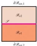Fig.1 Two examples of bidomain. Left. Both domains $\mathcal{B}{oi}$ have an external boundary $\partial \mathcal{B}{ext,i}$ and are separated each other by the interface $\mathcal{I}$ . Right. The domain $\mathcal{B}{o1}$ is inside $\mathcal{B}{o2}$ and its boundary is the interface $\mathcal{I}$ ; only the domain $\mathcal{B}{o2}$ has an external boundary $\partial \mathcal{B}{ext}$ . A domain $\mathcal{B}_{o2}$ , like that in the right panel, is called skin when its thickness is much smaller than a characteristic size of $\mathcal{B}_o$ .

As illustrated in Fig. 1, depending on the geometry, both domains may share an external boundary $\partial \mathcal{B}_{\mathrm{ext}}$ in contact with the environment (e.g., a stacked bi-layer, left panel), or one domain may act as an encapsulating skin such that only it possesses an external boundary (right panel). These distinct boundary definitions dictate where evaporative fluxes and convective heat transfer occur versus where internal mass and heat exchanges take place.

Since we consider a time-dependent problem, each field is defined on the space-time domain $\mathcal{B}_n\times \mathcal{T}$ , with $\mathcal{T} = (t_0,t_1)$ . The reference configuration is stress-free and characterized by uniform temperature and chemical potential. The state variables, including the reactive pressure, are

$\mathbf{u}\colon \mathcal{B}n\times \mathcal{T}\to \mathbb{V}$ displacement of $\mathcal{B}_o$ $[\mathbf{u}] = \mathfrak{m};$ c1: $\mathcal{B}{oi}\times \mathcal{T}\rightarrow \mathbb{R}$ concentration in $\mathcal{B}{oi}$ $[c{i}] = \mathrm{mol~m}^{-1}$ (1) $p\colon \mathcal{B}_n\times \mathcal{T}\to \mathbb{R}$ reactive pressure in $\mathcal{B}_o$ $[p] = \mathrm{Pa};$ T: $\mathcal{B}_o\times \mathcal{T}\to \mathbb{R}$ temperature in $\mathcal{B}_o$ $[T] = \mathbf{K};$

We recall that displacement and temperature are continuous throughout the reference domain $\mathcal{B}_o$ . In contrast, the water concentration and the pressure may be discontinuous across the interface $\mathcal{I}$ . Since we solve the problem using the weak form, spatial gradients of the concentration field enter the balance equations, whereas gradients of the pressure do not. Consequently, the concentration must belong to a function space that accommodates possible jumps across $\mathcal{I}$ . For this reason, we introduce two independent concentration fields, $c_1$ and $c_2$ , each defined on its respective subdomain. To avoid unnecessary notation, subscripts will be used only when the distinction between the two fields is essential.

The current position $x$ of a material point $X \in \mathcal{B}0$ at time $t$ is given by $x = X + \mathbf{u}(X,t) = f(X,t)$ , where $f$ is the motion; $\mathcal{B}_t = f(\mathcal{B}_0,t)$ is called current configuration. Given a reference frame ${o_1\mathbf{e}_1,\mathbf{e}_2,\mathbf{e}_3}$ , the displacement vector is represented by its components $\mathbf{u} = (u,v,w)$ ; analogously, any tensor $\mathbf{A}$ is represented with its components $A{ij} = \mathbf{A}\cdot \mathbf{e}_i\otimes \mathbf{e}_j$ .

Let $\mathrm{d}V$ and $\mathrm{d}v$ represent the reference and the current volume elements, respectively; analogously, let $\mathrm{d}A$ and $\mathrm{d}a$ be the reference and the current surface elements, respectively.

This journal is © The Royal Society of Chemistry 2026

Soft Matter, 2026, 22, 3238-3251

---

Soft Matter

Paper

Given the deformation gradient $\mathbf{F} = \nabla f$, the Jacobian $J = \operatorname*{det}\mathbf{F}$ and the cofactor $\mathbf{F}^{\star} = J\mathbf{F}^{-\mathrm{T}}$, we have the following geometric relations

\[\mathrm {d} v = J \mathrm {d} V, \quad \mathrm {d} a = \| \mathbf {F} ^ {\star} \mathbf {m} \| \mathrm {d} A, \quad \mathbf {n} = \frac {\mathbf {F} ^ {\star} \mathbf {m}}{\| \mathbf {F} ^ {\star} \mathbf {m} \|} \tag {2}\]

with $\mathbf{m}$ and $\mathbf{n}$ the normal vector to the reference boundary $\partial \mathcal{B}o$ and the current one $\partial \mathcal{B}_t$, respectively. The elementary water content $\mathrm{d}V{\mathrm{w}}$ is related to the molar concentration $c$ by $\mathrm{d}V_{\mathrm{w}} = \Omega c\mathrm{d}V$, where $\Omega = 1.8\times 10^{-5}\mathrm{m}^3\mathrm{mol}^{-1}$ is the molar volume of water.

2.2 Solid fraction and volumetric constraint

A key hypothesis of the Flory-Rehner theory states that any volume change of the swollen specimen is due to the change of its water content: this hypothesis couples mechanics - change in volume, to chemistry - change in solvent.

According to this hypothesis, within any volume element $\mathrm{d}V$ in $\mathcal{B}o$, we can identify the solid volume $\mathrm{d}V{\mathrm{s}}$ and the water volume $\mathrm{d}V_{\mathrm{w}}$. Similarly, in the current configuration $\mathcal{B}_t$, the volume element $\mathrm{d}v$ is the sum of its solid and water components:

\[\mathrm {d} v = \mathrm {d} v _ {\mathrm {s}} + \mathrm {d} v _ {\mathrm {w}}, \quad \mathrm {d} V = \mathrm {d} V _ {\mathrm {s}} + \mathrm {d} V _ {\mathrm {w}}. \tag {3}\]

Taking the ratio of the current and reference volume elements, which is measured by the Jacobian $J_{t}$, gives

\[\frac {\mathrm {d} v}{\mathrm {d} V} = J = \frac {\mathrm {d} v _ {\mathrm {s}}}{\mathrm {d} V} + \frac {\mathrm {d} v _ {\mathrm {w}}}{\mathrm {d} V}. \tag {4}\]

Assuming $\mathrm{d}v_{\mathrm{s}} = \mathrm{d}V_{\mathrm{s}}$ (solid is incompressible) and $\mathrm{d}v_{\mathrm{w}} = \Omega \mathrm{d}v_{\mathrm{s}}$ with $\Omega$ the molar volume of water (water volume is measured by concentration $c$), one obtains the volumetric constraint that couples mechanical deformations to water content:

\[J _ {i} = \frac {\mathrm {d} V _ {\mathrm {s}}}{\mathrm {d} V} + \Omega c _ {i} = \phi_ {o i} + \Omega c _ {i}, \tag {5}\]

with $\phi_{oi}$ the initial solid fraction of $\mathcal{B}_{oi}$. The current solid fraction $\phi_i$ in $\mathcal{B}_t$ is given by

\[\phi_ {i} = \frac {\mathrm {d} V _ {\mathrm {s}}}{\mathrm {d} v} = \frac {\phi_ {o i} \mathrm {d} V}{\left(\phi_ {o i} + \Omega c _ {i}\right) \mathrm {d} V} = \frac {\phi_ {o i}}{\phi_ {o i} + \Omega c _ {i}} = \frac {\phi_ {o i}}{J _ {i}}. \tag {6}\]

The total change of water volume $V_{\mathrm{w}}(t)$ at time $t$ is given by

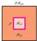
\[V _ {\mathrm {w}} (t) = \int_ {\mathcal {B}} (J (t) - 1) \mathrm {d} V. \tag {7}\]

Let $\mathcal{B}{gi}$ be the ground configuration of $\mathcal{B}{oi}$, that is the fully dry states that the domain $\mathcal{B}{oi}$ would attain if it were physically separated by a cut prior to drying; the deformation from ground $\mathcal{B}{gi}$ to current $\mathcal{B}t$ is measured by $\mathbf{F}{\mathrm{e}} = \mathbf{F}\mathbf{F}{\mathrm{eo}}$, where $\mathbf{F}{\mathrm{eo}} = J_{\mathrm{ov}}^{1 / 3}\mathbf{I}$ is the deformation from ground to initial $\mathcal{B}{oi}$. Relations between deformations $\mathbf{F}$, $\mathbf{F}{\mathrm{ei}}$, $\mathbf{F}{\mathrm{eoi}}$, their Jacobians $J, J{\mathrm{ei}}, J_{\mathrm{eoi}}$ and volume fractions $\phi_i, \phi_{oi}$ are shown in Fig. 2.

2.3 Free energy

Following the thermodynamic framework for swelling gels, $^{19,35}$ extended to poly-domains gels in ref. 12, we consider a mixing energy $\psi_{\mathrm{m}}$ per unit of current volume $\mathrm{d}v$, and an elastic energy

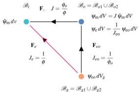Fig. 2 The three states scheme. Ground state $\mathcal{B}{gi}$ swells to initial configuration $\mathcal{B}{oi}$: upon drying, the initial configuration $\mathcal{B}o$ deforms to the current one $\mathcal{B}_t$. The current configuration $\mathcal{B}_t$ is described by the displacement $\mathbf{u}$ from $\mathcal{B}_o$. The elementary energy densities $\psi{\mathrm{m}}\mathrm{d}V$ (mixing) and $\psi_{\mathrm{eo}}\mathrm{d}V_{\mathrm{g}}$ (elastic) are defined on $\mathcal{B}t$ and $\mathcal{B}{gi}$ respectively. Their reference counterparts $\psi_{\mathrm{m}}\mathrm{d}V$ and $\psi_{\mathrm{e}}\mathrm{d}V$ are defined on $\mathcal{B}_o$. Subscripts $i$ are omitted.

$\psi_{\mathrm{eo}}$ per unit of ground volume $\mathrm{d}V_{\mathrm{g}}$, see Fig. 2. The total free energy $\psi (\mathbf{F}_{\mathrm{e}},\phi)$ per unit of reference volume $\mathrm{d}V$ is given by

\[\psi \left(\mathbf {F} _ {\mathrm {e}}, \phi\right) = \psi_ {\mathrm {e}} \left(\mathbf {F} _ {\mathrm {e}}\right) + \psi_ {\mathrm {m}} (\phi) = \frac {1}{J _ {\mathrm {e o}}} \psi_ {\mathrm {e o}} \left(\mathbf {F} _ {\mathrm {e}}\right) + J \hat {\psi} _ {\mathrm {m}} (\phi). \tag {8}\]

For mixing, we consider the Flory-Huggins energy $\hat{\psi}_{\mathrm{m}}$ given by

\[\hat {\psi} _ {\mathrm {m}} (\phi) = \frac {R T}{\Omega} \left[ (1 - \phi) \log (1 - \phi) + \chi \phi (1 - \phi) \right], \tag {9}\]

where $\chi$ is the Flory parameter, and $R$ the gas constant. For elasticity, we assume the neo-Hookean energy $\psi_{\mathrm{eo}}$ given by

\[\psi_ {\mathrm {e o}} \left(\mathbf {F} _ {\mathrm {e}}\right) = \frac {1}{2} G \left(\mathbf {F} _ {\mathrm {e}} \cdot \mathbf {F} _ {\mathrm {e}}\right) - 3), \tag {10}\]

with $G$ the shear modulus. Finally, we include the volumetric constraint into the energy by adding a pressure term $p$ acting as Lagrange multiplier; this defines the relaxed energy $\psi_{\mathrm{R}}$:

\[\psi_ {\mathrm {R}} \left(\mathbf {F} _ {\mathrm {e}}, \phi\right) = \frac {1}{J _ {\mathrm {e o}}} \psi_ {\mathrm {e o}} \left(\mathbf {F} _ {\mathrm {e}}\right) + J \hat {\psi} _ {\mathrm {m}} (\phi) - p [ J - \left(\phi_ {\mathrm {o}} + \Omega c\right) ] \tag {11}\]

The time derivative of the free energy (11) yields the constitutive relations for the reference stress $\mathbf{S}$ (first Piola-Kirchhoff stress), the chemical potential $\mu$, and the water flux $\mathbf{j}$; we have

\[\dot {\psi} _ {\mathrm {R}} = \frac {1}{J _ {\mathrm {e o}}} \frac {\partial \psi_ {\mathrm {e o}}}{\partial \mathbf {F}} \cdot \dot {\mathbf {F}} + \frac {\partial}{\partial \phi} \left(\frac {\phi_ {\mathrm {o}}}{\phi} \hat {\psi} _ {\mathrm {m}}\right) \dot {\phi} - p \dot {J} + p \Omega \dot {c}. \tag {12}\]

Note that in the second summand of (12), representing the mixing contribution, $J$ is written as function of the solid fraction: $J = \phi_{\mathrm{o}} / \phi$; analogously, also the concentration rate $\dot{c}$ can be represented in terms of $\phi$. All the details about the derivation of the constitutive relations from (12) can be found in ref. 12.

Soft Matter, 2026, 22, 3238-3251

This journal is © The Royal Society of Chemistry 2026

---

Paper

Soft Matter

2.4 Balance of forces

We assume that inertia forces are negligible, and bulk forces are zero. The balance of linear momentum is expressed as

\[\operatorname {d i v} \mathbf {S} = 0 \quad \text {o n} \mathcal {B} _ {\mathrm {o}} \times \mathcal {F}, \quad \mathbf {S m} = \mathbf {t} \quad \text {o n} \partial \mathcal {B} _ {\mathrm {o}} \times \mathcal {F}, \tag {13}\]

where $\mathbf{S}$ is the reference stress and $\mathbf{t}$ is the nominal traction acting on the boundary $\partial \mathcal{B}_0$ . From (10) and (11), it follows the formula for the reference stress $\mathbf{S}$ and the current (Cauchy) stress $\mathbf{T}$ :

\[\mathbf {S} = \phi_ {\mathrm {e r}} ^ {- 1 / 3} G _ {i} \mathbf {F} - p \mathbf {F} ^ {*}, \quad \mathbf {T} = \frac {1}{J} \mathbf {S} \mathbf {F} ^ {\mathrm {T}} = \frac {\phi_ {\mathrm {e i}} ^ {- 1 / 3}}{J} G _ {i} \mathbf {F} \mathbf {F} ^ {\mathrm {T}} - p \mathbf {I}. \tag {14}\]

2.5 Balance of water mass

The total mass of water changes only because water can enter or exit in the specimen through its boundary; the balance of mass writes as

\[\dot {c} _ {i} + \operatorname {d i v} \mathbf {j} _ {i} = 0 \quad \text {o n} \mathcal {B} _ {\mathrm {o} i} \times \mathcal {F}, \quad - \mathbf {j} _ {i} \cdot \mathbf {m} = s _ {\mathrm {w} i} \quad \text {o n} \partial \mathcal {B} _ {\mathrm {o} i} \times \mathcal {F}, \tag {15}\]

where $\mathbf{j}i$ is the molar flux of water and $s{\mathrm{wi}}$ the boundary source, $[\mathbf{j}i] = [s{\mathrm{wi}}] = \mathrm{mol}(\mathrm{m}^{-2}\mathrm{s}^{-1})$ . The flux $\mathbf{j}_i$ is related to the chemical potential $\mu_i$ by the constitutive law

\[\mathbf {j} _ {i} = - \mathbf {M} _ {i} \nabla \mu_ {i}, \quad \text {w i t h} \quad \mathbf {M} _ {i} = \frac {D c _ {i}}{R T} \mathbf {C} ^ {- 1}, \mathbf {C} = \mathbf {F} ^ {\mathrm {T}} \mathbf {F}. \tag {16}\]

with $D$ the water diffusivity, $[D] = \mathrm{m}^2\mathrm{s}^{-1}$ and $R$ the universal gas constant, $[R] = \mathbf{J}(\mathrm{mol~K})^{-1}$ . The chemical potential $\mu_{i}$ is derived from (9) and the energy rate (12); we have

\[\mu_ {i} = R T \left(\log \left(1 - \phi_ {i}\right) + \phi_ {i} + \chi \phi_ {i} ^ {2}\right) + \Omega p, [ \mu_ {i} ] = J m o l ^ {- 1}, \tag {17}\]

where $\chi = \chi_{\mathrm{eff}}(T,\phi_i)$ is the effective Flory parameter, possibly depending on temperature and solid fraction of domain $i$ .

2.5.1 Temperature dependent Flory-Huggins parameter

Here we assume $\chi$ to be primarily sensitive to temperature $T$ and, to a lesser extent, to the solid fraction $\phi$ ; we employ the following constitutive law:

\[\chi_ {\text {e f f}} (T, \phi) = \chi_ {0} + (\bar {\chi} (T) - \chi_ {0}) \phi^ {2} \tag {18}\] \[\bar {\chi} (T) = \chi_ {1} + (\chi_ {\infty} - \chi_ {1}) \sigma (T)\]

with $\sigma (T) = 1 / [1 + a\exp (-b(T - T_{\mathrm{d}}))]$ the sigmoid function; the parameters $a = 10$ and $b = 0.5~1 / \mathrm{K}$ are such that $\sigma (T_{\mathrm{d}})\simeq 1 / 2$ , at $T_{\mathrm{d}} = 323\mathrm{K}$ the transition temperature. From (18), it follows

\[\chi_ {\text {e f f}} (T, \phi) \simeq \left\{ \begin{array}{l l} \chi_ {0}, & \text {f o r} \phi \ll 1 (\text {h i g h l y s w o l l e n}) \\ \bar {\chi} (T), & \text {f o r} \phi \simeq 1 (\text {a l m o s t d r y}) \end{array} \right. \tag {19}\]

Moreover, we note that for $T \ll T_{\mathrm{d}}$ , we have

\[\bar {\chi} (T) = \chi_ {1}, \quad \chi_ {\text {e f f}} (T, \phi) = \chi_ {0} + \left(\chi_ {1} - \chi_ {0}\right) \phi^ {2} \tag {20}\]

that is, $\chi_0$ and $\chi_{1}$ represent the values of the Flory parameter at low temperature, that is before denaturation, for the highly swollen and the almost dry state, respectively. The temperature and composition dependency of the Flory-Huggins interaction parameter specified by (18) has been used $^{36}$ to model the denaturation of meat proteins, but can describe many

biopolymers and thermoresponsive hydrogels. $^{11,37,37}$ For biopolymers, $^{37}$ it is often chosen the value $\chi_{\mathrm{o}} = 0.5$ , corresponding to the critical value of semi-dilute regime; this value is based on the assumption that near room temperature, water acts as a good-solvent.

2.5.2 Boundary conditions for water flux

The boundary of each domain $\partial \mathcal{B}{\mathrm{oi}}$ is made of an external boundary $\partial \mathcal{B}{\mathrm{ext}}$ , plus the boundary with the adjacent domain, called interface $\mathcal{S}$ . We describe the water source $s_w$ at the boundary by using a molar flux, product of a mass transmission coefficient $(\mathrm{ms}^{-1})$ times a molar density $(\mathrm{mol~m}^{-3})$

\[s _ {\mathrm {w}} = \text {m o l a r f l u x} = \text {t r a n s m i s s i o n c o e f f i c i e n t} \times \text {m o l a r d e n s i t y}. \tag {21}\]

A different approach is used to determine molar density at the external boundary $\partial \mathcal{B}_{\mathrm{ext},i}$ versus at the interface $\mathcal{S}_i$ between two domains.

2.5.2.1 External boundary

At $\partial \mathcal{B}{\mathrm{ext},i}$ , both temperature and chemical potential might have a jump. On the internal side of the boundary, the chemical potential of the vapor phase is equal to $\mu{i}$ , the chemical potential of the solid at the surface, given by (17). Treating the vapor-air mixture as a solution of ideal gases, the vapor concentration $c_{\mathrm{v}}$ of the external vapor phase at direct contact with the boundary is related to its chemical potential $\mu_{i}$ by the ideal gas law:

\[\mu_ {i} = R T \log \left(\frac {c _ {\mathrm {v}}}{c _ {\mathrm {s a t}} \left(T _ {\mathrm {e x t}}\right)}\right). \tag {22}\]

This relation can be inverted to express the vapor concentration at the material surface as a function of its chemical potential:

\[c _ {\mathrm {v}} = a _ {\mathrm {w}} c _ {\mathrm {s a t}} \left(T _ {\mathrm {e x t}}\right) \quad \text {w i t h} \quad a _ {\mathrm {w}} = \exp \left(\frac {\mu_ {i}}{R T}\right), \tag {23}\]

where $a_{\mathrm{w}}$ represents the water activity at the boundary, a quantity of common use in physical chemistry to express concentration.

The same law governs the relation between chemical potential $\mu_{\mathrm{ext}}$ and vapor concentration $c_{\mathrm{v,ext}}$ at the external side of the boundary:

\[\mu_ {\mathrm {e x t}} = R T _ {\mathrm {e x t}} \log \left(\frac {c _ {\mathrm {v , e x t}}}{c _ {\mathrm {s a t}} \left(T _ {\mathrm {e x t}}\right)}\right). \tag {24}\]

Unlike $c_{\mathrm{v}}$ , the vapor concentration $c_{\mathrm{v,ext}}$ is experimentally accessible, and is usually written as a fraction of the saturation concentration $c_{\mathrm{sat}}(T_{\mathrm{ext}})$ at the external temperature $T_{\mathrm{ext}}$ through the relative humidity of the air $\mathrm{RH}_{\mathrm{air}}$ :

\[c _ {\mathrm {v}, \text {e x t}} = \mathrm {R H} _ {\text {a i r}} c _ {\text {s a t}} \left(T _ {\text {e x t}}\right). \tag {25}\]

The saturated vapour concentration is related to the saturated vapour pressure $p_{\mathrm{sat}}$ , with $[p_{\mathrm{sat}}] = \mathrm{Pa} = \mathrm{J} \, \mathrm{m}^{-3}$ , by

\[c _ {\text {s a t}} (T) = M _ {\mathrm {w}} \frac {\rho_ {\text {s a t}} (T)}{R T}, \quad \left[ \frac {p _ {\text {s a t}}}{R T} \right] = \mathrm {m o l} \, \mathrm{m} ^ {- 3}. \tag {26}\]

This journal is © The Royal Society of Chemistry 2026

Soft Matter, 2026, 22, 3238-3251

---

The saturated vapour pressure p_{sat} is given by a variant of the Magnus–Tetens equation, which gives a convenient and accurate fit for temperatures near and above freezing:

This formula is valid when temperature is expressed in Celsius degrees; thus, the difference T - T_{ref}, with T_{ref} = 273.15 K, rescales Kelvin to Celsius; the empirical constant 610.78 Pa is the vapor pressure at 0 °C. The constants 17.27 and 237.3 °C are chosen from ref. 6 so that the formula matches experimental data for liquid water between about 0 °C and +100 °C, with a max error of 0.1%.

Convective mass transfer across the boundary is driven by the jump in chemical potential

$\Delta\mu=\mu_{\text{ext}}-\mu_{i}.$ (28)

Nevertheless, common engineering practice^{38,39} quantifies departure from equilibrium through the jump in molar density Δn_{v}, represented by

$\Delta\mu=\frac{\Delta c_{\text{v}}}{M_{\text{w}}}=\frac{c_{\text{v,ext}}-c_{\text{v}}}{M_{\text{w}}},\quad\left

\Delta c_{\text{v}}\right

=\text{Kg m}^{-3},$ (29)

where M_{w} is the molar mass of water ([M_{w}] = Kg mol^{-1}). The two points of view can be reconciled by noting that, in the range of temperatures and concentrations relevant for our problem, the chemical potential is more sensitive to changes in concentration than to changes in temperature, thus, the jump of chemical potential can approximated as

$\Delta\mu\approx\left(\frac{\partial\mu}{\partial c_{\text{v}}}\right){\text{T}}\Delta c{\text{v}}.$ (30)

Within the scope of the above approximation, the boundary source term s_{wi} is assumed to be both temperature dependent and proportional to the molar density Δn_{v} through the relation

$s_{wi}(T)=A\beta_{i}\frac{\Delta c_{\text{v}}}{M_{\text{w}}}\quad\text{on}\quad\partial\mathscr{B}_{\text{ext},i}\times\mathcal{F},$ (31)

where β_{i} is the mass transfer coefficient for the external surface ([β_{i}] = m s^{-1}) and A = ∥F*m∥ the ratio dα/dA of area change between reference and current state, which takes into account the effect of deformation on the mass transfer across boundary.

Interface

Molar density at the interface 𝒪_{i} separating two domains is determined by the difference in chemical potentials Δμ_{i} across the interface; being [RT] = J mol^{-1}, we have

$\text{Molar density}=\frac{\Delta\mu_{i}}{RT\Omega},\quad\left[\frac{\Delta\mu_{i}}{\Omega}\right]=\text{J m}^{-3}.$ (32)

The water source s_{wi} at 𝒪_{i} is given by

$s_{wi}=A\beta_{\text{v}}\frac{\Delta\mu_{i}}{RT\Omega}\quad\text{on}\quad\partial\mathcal{G}_{i}\times\mathcal{F}$ (33)

where β_{s} is the mass transfer coefficient ([β_{s}] = m s^{-1}) at the interface, defined by β_{s} = D/ξ with ξ an effective thickness ([ξ] = m); the jump Δμ_{i} is given

$\Delta\mu_{1}=\mu_{2}-\mu_{1},\quad\Delta\mu_{2}=\mu_{1}-\mu_{2}.$ (34)

Remark

It is worth noting that relation (31) and (33) have the same structure; in particular, the ratio Δc_{v}/M_{w} has the same role of Δμ_{i}/(RTΩ). Actually in the present model, the air–vapor mixture is modeled as a solution of ideal gases. Accordingly, the chemical potential of the external vapor phase is

$\mu_{\text{ext}}=RT_{\text{ext}}\log\left(\frac{p_{\text{v,ext}}}{p_{\text{sat}}(T_{\text{ext}})}\right),$ (35)

where p_{sat}(T_{ext}) denotes the saturation pressure of vapor at temperature T_{ext}. In writing (35), it is understood that the reference value for chemical potential is that of water at temperature T_{ext}, because at this temperature water is in equilibrium with its vapor at the pressure p_{sat}(T_{ext}). Since the partial pressure p_{v,ext} of water vapor is related to its molar concentration c_{v,ext}/M_{w} by the equation of state $p_{\text{v,ext}}=\frac{c_{\text{v,ext}}}{M_{\text{w}}}RT_{\text{ext}}$, we can rewrite (35) as

$\mu_{\text{ext}}=RT_{\text{ext}}\log\left(\frac{c_{\text{v,ext}}}{c_{\text{sat}}(T_{\text{ext}})}\right)=RT_{\text{ext}}\log(\text{RH}_{\text{air}}),$ (36)

an expression that involves the variables that control the drying process, namely, the relative humidity RH_{air} of the air and its temperature T_{ext}. If T = T_{ext}, then, by (23) and (25), we have

$\mu_{\text{ext}}-\mu_{i}=RT_{\text{ext}}\log\left(\frac{c_{\text{v,ext}}}{c_{\text{v}}}\right).$ (37)

Thus, when T = T_{ext}, the variable c_{v} is the vapor concentration at which Δμ = μ_{ext} - μ_{i} = 0, so that air and gel would be in chemical equilibrium. Although the quantity Δc_{v} = c_{ext} - c_{v} is not observable, it is instrumental for quantifying departure from interfacial chemical equilibrium. In fact, if T = T_{ext}, then

$\Delta\mu=RT_{\text{ext}}\log\left(1+\frac{\Delta c_{\text{v}}}{c_{\text{v}}}\right)\approx RT_{\text{ext}}\frac{\Delta c_{\text{v}}}{c_{\text{v,ext}}}.$ (38)

where the error is controlled by

Δc_{v}/c_{v,ext}

. If T_{ext} ≠ T an extra error is introduced in (38) which is controlled by

(T_{ext} - T)/T_{ext}

.

Heat transfer

Let U be the internal energy per unit reference volume. The first law of thermodynamics states that the time rate of internal energy is balanced by the mechanical power and the divergence of the total energy flux:

$\dot{U}=\mathbf{S}:\mathbf{F}-\text{div }\mathbf{q},$ (39)

where the total energy flux, namely,

$\mathbf{q}=\mathbf{q}{\text{c}}+h{\text{w}}\mathbf{j},$ (40)

is assumed to be the sum of a conductive term q_{c} and a convective one h_{w}j, with h_{w} the specific enthalpy of water (recall that j is the molar flux of water).

---

Paper

Soft Matter

Adding to the free-energy density $\psi_{\mathrm{R}}$ a thermal contribution, we represent the internal energy as $U = \psi_{\mathrm{R}} + TS$, with $S$ the entropy density; thus, the balance of power writes as

\[\frac {\partial \psi_ {\mathrm {R}}}{\partial \dot {\mathbf {F}}} \cdot \dot {\mathbf {F}} + \frac {\partial \dot {\psi} _ {\mathrm {R}}}{\partial \phi} \dot {\phi} + \frac {\partial \dot {\psi} _ {\mathrm {R}}}{\partial T} \dot {T} + S \dot {T} + T \dot {S} = \mathbf {S} \cdot \dot {\mathbf {F}} - \operatorname {d i v} \mathbf {q}. \tag {41}\]

As noticed in Section 2.3, the first two summands of free energy rate $\dot{\psi}$ yield the constitutive eqn (14) and (17) for stress $\mathbf{S}$ and chemical potential $\mu$, together with the swelling constraint $J = \phi_{0} + \Omega c$; thus, we obtain a reduced balance equation

\[\frac {\partial \psi_ {\mathrm {R}}}{\partial T} \dot {T} + \dot {T} S + T \dot {S} + \mu \dot {c} = - \operatorname {d i v} \mathbf {q}. \tag {42}\]

Now, we expand the rate of entropy change using the chain rule, the Maxwell relations $\frac{\partial S}{\partial \dot{\mathbf{F}}} = -\frac{\partial \mathbf{S}}{\partial T}$, and $\frac{\partial S}{\partial c} = -\frac{\partial \mu}{\partial T}$, and the relation $\frac{\partial \Psi}{\partial T} = -S$, and recalling that $\dot{c} = -\mathrm{div} \, \mathbf{q}$, we arrive at

\[T \frac {\partial S}{\partial T} \dot {T} + T \frac {\partial \mathbf {S}}{\partial T} \cdot \dot {\mathbf {F}} = \left(\mu - \frac {\partial \mu}{\partial T}\right) \operatorname {d i v} \mathbf {j} - \operatorname {d i v} \mathbf {q}. \tag {43}\]

From fundamental thermodynamics, enthalpy is related to chemical potential and entropy by $h_{\mathrm{w}} = \mu + T \ddot{s}{\mathrm{w}}$, where the partial molar entropy is $\ddot{s}{\mathrm{w}} = -\frac{\partial \mu}{\partial T}$. Therefore, the term in parentheses is exactly the partial molar enthalpy:

\[\mu - T \frac {\partial \mu}{\partial T} = h _ {\mathrm {w}}. \tag {44}\]

As a result, recalling (40), the energy balance can be written as

\[T \frac {\partial S}{\partial T} \dot {T} - T \frac {\partial \mathbf {S}}{\partial T} \cdot \dot {\mathbf {F}} = - \operatorname {d i v} \left(\mathbf {q} _ {\mathrm {c}} + h _ {\mathrm {w}} \mathbf {j}\right). \tag {45}\]

We approximate the effective heat capacity $C_{\mathrm{eff}} = T\frac{\partial S}{\partial T}$ with a constant $[C_{\mathrm{eff}}] = \mathrm{J}(\mathrm{m}^{-3}\mathrm{K}^{-1})$, which we express as $C_{\mathrm{eff}} = \rho_{\mathrm{p}}c_{\mathrm{p}}$, where $\rho_{\mathrm{p}}$ the mass density, $[\rho_{\mathrm{p}}] = \mathrm{Kg}\mathrm{m}^{-3}$, and $c_{\mathrm{p}}$ the specific heat, $[c_{\mathrm{p}}] = \mathrm{J}(\mathrm{Kg}\mathrm{K})^{-1}$. Furthermore, we neglect thermoelastic effects by discarding the second term on the left-hand side of (45), which is justified by the fact that the change in entropy with respect to deformation is typically much smaller than the change in entropy with respect to temperature. With these approximations, the energy balance simplifies to

\[J C _ {\text {e f f}} \dot {T} + \operatorname {d i v} \mathbf {q} = 0, \quad \text {on} \mathcal {B} _ {\mathrm {o}} \times \mathcal {F}, \tag {46}\]

which is supplemented by the boundary condition

\[- \mathbf {q} \mathbf {m} = s _ {\mathrm {h}}, \quad \text {on} \partial \mathcal {B} _ {\mathrm {o}} \times \mathcal {F}, \tag {47}\]

where $s_{\mathrm{h}}$ the boundary source of heat, with $[\mathbf{q}] = [s_{\mathrm{h}}] = \mathbf{W} \, \mathrm{m}^{-2}$.

Finally, assuming that the conductive heat flux obeys the Fourier’s law:

\[\mathbf {q} _ {\mathrm {c}} = - k _ {\mathrm {p}} \nabla T, \tag {48}\]

where $k_{\mathrm{p}}$ is the thermal conductivity, $[k_{\mathrm{p}}] = \mathrm{W}(\mathrm{mK})^{-1}$, and that specific enthalpy of water is proportional to temperature:

\[h _ {\mathrm {w}} = \Omega C _ {\mathrm {w}} T, \tag {49}\]

with $C_{\mathrm{w}} = \rho_{\mathrm{w}}c_{\mathrm{w}}$ is the water volumetric heat capacity, $[C_{\mathrm{w}}] = \mathrm{J}(\mathrm{m}^{-3}\mathrm{K}^{-1})$, with $\rho_{\mathrm{w}}$ the water mass density, $[\rho_{\mathrm{w}}] = \mathrm{Kg}\mathrm{m}^{-3}$, and $c_{\mathrm{w}}$ the specific heat of water, $[c_{\mathrm{w}}] = \mathrm{J}(\mathrm{Kg}\mathrm{K})^{-1}$, we obtain

\[\mathbf {q} = - k _ {\mathrm {p}} \nabla T + \Omega C _ {\mathrm {w}} T \mathbf {j}. \tag {50}\]

2.7 Boundary conditions for heat transfer

The boundary conditions for heat transfer are the surface counterpart of the bulk energy balance derived in the previous section: at the external surface $\partial \Omega_{\mathrm{ext}}$, the net heat flux $\mathbf{q} \cdot \mathbf{n}$ must equal the sum of convective heat exchange with the surrounding air and the latent heat released by evaporating water. Following the standard treatment of convective drying,[38-40] we decompose the boundary heat source as:

\[s _ {\mathrm {h i}} = s _ {\mathrm {h c}} + s _ {\mathrm {h w i}}, \quad [ \mathrm {s h i} ] = \mathrm {W m} ^ {- 2}. \tag {51}\]

2.7.1 Convective heat exchange

The convective term follows Newton’s law of cooling.[29] Pulled back to the reference configuration using the area stretch ratio $A = | \mathbf{F}^{*}\mathbf{m}|$, it reads:

\[s _ {\mathrm {h c}} (T) = A h _ {\mathrm {a i r}} \left(T _ {\mathrm {e x t}} - T\right), \tag {52}\]

with $h_{\mathrm{air}}$ the convective heat transfer coefficient, $^{39}$ $[h_{\mathrm{air}}] = \mathrm{W}(\mathrm{m}^{-2}\mathrm{K}^{-1})$. The factor $A$ accounts for the deformation of the surface in the current configuration relative to the reference one.

In the soft domain, the convective heat transfer coefficient $h_{\mathrm{air}}$ and the mass transfer coefficient $\beta$ are related through the Lewis relation:39,40

\[\beta = \frac {h _ {\text {a i r}}}{\rho_ {\text {a i r}} c _ {\mathrm {p} , \text {a i r}}}, \tag {53}\]

which reflects the analogy between heat and mass transfer in a turbulent boundary layer. This gives $\beta_{1} = 0.0132 \, \mathrm{m} \, \mathrm{s}^{-1}$ in the soft domain; a smaller value $\beta_{2} = 10^{-4} \, \mathrm{m} \, \mathrm{s}^{-1}$ is assigned to the stiffer domain, consistent with its reduced surface permeability.

2.7.2 Evaporative heat

When water escapes through the surface, it carries away its molar latent heat of evaporation $L_{\mathrm{v}}(T)$. This evaporative cooling is the direct thermodynamic cause of the wet-bulb effect:

\[s _ {\mathrm {h w i}} (T) = s _ {\mathrm {w i}} (T) L _ {\mathrm {v}} (T), \tag {54}\]

where a negative $s_{\mathrm{wi}}$ results in a heat sink effect.38 Note that this term is the surface counterpart of the convective enthalpy flux $C_{\mathrm{w}}T\mathbf{j}$ appearing in the definition of $\mathbf{q}$, see eqn (50); water migrating in the bulk carries sensible heat; at the surface, the phase change additionally releases latent heat.

The temperature-dependent latent heat is given by:

\[L _ {\mathrm {v}} (T) = \Delta H _ {\mathrm {r}} ^ {\mathrm {e a p}} + \left(c _ {\mathrm {p}, \mathrm {v}} - c _ {\mathrm {p}, \mathrm {i}}\right) \left(T - T _ {\mathrm {r}}\right), \quad \left[ L _ {\mathrm {v}} \right] = \mathrm {J} \mathrm {m o l} ^ {- 1}. \tag {55}\]

$\Delta H_{\mathrm{exp}}^{\prime}$ is the latent heat of evaporation at reference temperature $T_{\mathrm{r}}$ with $[\Delta H_{\mathrm{exp}}] = \mathrm{J} \, \mathrm{mol}^{-1}$; $c_{\mathrm{p,v}}$ and $c_{\mathrm{p,i}}$ are the molar heat capacities of vapor and liquid, respectively (assumed constant

This journal is © The Royal Society of Chemistry 2026

Soft Matter, 2026, 22, 3238-3251

---

Soft Matter

Paper

with temperature), with $[c_{\mathrm{p,v}}] = [c_{\mathrm{p,i}}] = \mathbf{J}(\mathrm{mol~K})^{-1}$. We set

$T_{\mathrm{r}} = 373.15\mathrm{K},$ reference temperature

$\Delta H_{\mathrm{cap}}^{\mathrm{r}} = 40.65\mathrm{KJ mol}^{-1},$ latent heat at $T_{\mathrm{r}}$ (56)

$c_{\mathrm{p,v}} = 34.6\mathrm{J}(\mathrm{mol~K})^{-1}$ vapor heat capacity,

$c_{\mathrm{p,i}} = 75.6\mathrm{J}(\mathrm{mol~K})^{-1}$ liquid water heat capacity.

Molar heat capacity $c_{\mathrm{p,v}}$, mass heat capacity $c_{\mathrm{p,v}}^{\mathrm{m}}$ and volume heat capacity $c_{\mathrm{p,v}}^{\mathrm{v}}$ are related by

\[c _ {\mathrm {p}, \mathrm {v}} ^ {\mathrm {m}} = \frac {c _ {\mathrm {p} , \mathrm {v}}}{M _ {\mathrm {w}}}, \quad c _ {\mathrm {p}, \mathrm {v}} ^ {\mathrm {v}} = \rho_ {\mathrm {v}} c _ {\mathrm {p}, \mathrm {v}} ^ {\mathrm {m}} = \frac {c _ {\mathrm {p} , \mathrm {v}}}{M _ {\mathrm {w}}}, \tag {57}\]

with $[c_{\mathrm{p,v}}^{\mathrm{mass}}] = \mathbf{J}(\mathrm{kg~K})^{-1}$, and $[c_{\mathrm{p,v}}^{\mathrm{vol}}] = \mathbf{J}(\mathrm{m}^{-3}\mathrm{K}^{-1})$.

2.8 Couplings

It is worth listing the many couplings between the model variables: (1) mechanical displacement and water content are coupled by the volumetric constraint (5). (2) Water content and temperature are coupled in many ways: the chemical potential is a function of $T$, see eqn (17) and (18); water flux at boundary is a function of $T$, see eqn (31) heat flux at boundary has a term depending on water flux, see eqn (51).

We emphasize that, since the reference configuration is taken to be a stress-free swollen state, the material parameters $G_{i}$ and $\chi$, the external chemical potential $\mu_{\mathrm{o}}$, and the initial solid fraction $\phi_{oi}$ are not independent. In particular, the stress-free equilibrium condition imposes a constraint among these quantities. Consequently, only three of the four parameters $G_{i}, \chi, \mu_{\mathrm{o}}$, and $\phi_{oi}$ may be prescribed independently, while the remaining one must be determined from the equilibrium condition.

For a given uniform chemical potential $\mu_{\mathrm{o}}$, differences in the shear moduli $(G_{i})$ lead to corresponding differences in the initial solid fraction $(\phi_{oi})$. Consequently, upon drying, this heterogeneity will induce differential de-swelling, yielding shape changes and mechanical frustration.

Specifically, Fig. 3 schematically illustrates how two domains with different stiffnesses $(G_{1} \neq G_{2})$ will inherently hold different equilibrium water volumes in their free-swollen state. When forced to undergo uniform drying, the softer, more hydrated domain undergoes a larger volumetric shrinkage than the stiffer domain. Because the two domains are kinematically bound at their interface, this differential shrinkage cannot be accommodated freely, leading to internal residual stresses, bending, and macroscopic shape morphing (mechanical frustration).

2.9 The initial state

We aim to characterize a generic material response, rather than calibrate the model to a particular material. Accordingly, we rely on a standard experimental protocol in which temperature, equilibrium water content, and the chemical potential of the external environment are independently controlled or measured.

We emphasize the distinction between the ground state and the initial state. The ground state $\mathcal{B}_{gi}$ is a hypothetical, fully dry,

Fig. 3 Drying incompatibility. Each square represents a unit volume: azure is water and plaster or coral is solid. Two dry specimen made of a soft (plaster) and a stiff (coral) solid matrix, have different shear moduli $G_{i}$ (top). Two same free swollen volumes $\mathcal{B}{oi}$ have different initial solid fractions $\phi{oi}$, thus containing different volumes of water. Upon drying, their final volumes will be different; by glueing the $\mathcal{B}{o1}$ to $\mathcal{B}{o2}$, it is not possible to have a stress free dry configuration (bottom).

and stress-free state for each disconnected domain $\mathcal{B}_{oi}$, which can only be reached by physically separating the two domains prior to drying. In contrast, the initial state $\mathcal{B}_0$ is the actual, physically connected, and fully swollen configuration, that we assume as reference (prior to the heating process).

The initial state is described by the initial value of the four state variables (1):

\[\mathbf {u} _ {\mathrm {o}} = \mathbf {u} (X, 0), \quad T _ {\mathrm {o}} = T (X, 0), p _ {o i} = p (X, 0), c _ {o i} = c (X, 0). \tag {58}\]

These initial values are determined by the following assumptions:

• $\mathcal{B}0 = \mathcal{B}{01} \cup \mathcal{B}_{02}$ is a free swelling state at uniform $\mu_0$;
• $\phi_{oi}$, the initial solid fraction of domain $\mathcal{B}_{oi}$, is known;
• $T_{\mathrm{o}}$, the initial temperature, is known.

As $\mathcal{B}0$ is also the reference configuration, we have $\mathbf{u}_0 = 0$ and $\mathbf{F}(X,0) = \mathbf{I}$; the elastic deformation from dry is measured by $\mathbf{F}{\mathrm{ei}} = \mathbf{F}\mathbf{F}{\mathrm{eoi}}$, where $\mathbf{F}{\mathrm{eoi}} = \lambda_{\mathrm{eoi}}\mathbf{I}$ is its initial value and $\lambda_{\mathrm{eoi}} = \phi_{\mathrm{oi}}^{-1 / 3}$. The free swelling condition at uniform $\mu_0$ requires that, for each domain $\mathcal{B}_{oi}$, the following equations are true

\[\dot {\mu} \left(\phi_ {o i}\right) + p _ {o i} \Omega = \mu_ {0} \quad \text {chemical equilibrium},\] \[\dot {\mathbf {T}} \left(\mathbf {F} _ {\mathrm {e o i}}\right) - p _ {\mathrm {o i}} \mathbf {I} = - p _ {\mathrm {a t m}} \mathbf {I} \quad \text {mechanical equilibrium}, \tag {59}\] \[\phi_ {o i} = 1 / J _ {e o i} \quad \text {volumetric constraint},\]

From (5), the initial liquid concentration $c_{oi}$ is given

\[c _ {o i} = \frac {1 - \phi_ {o i}}{\Omega}. \tag {60}\]

From (18), we have $\chi_{oi} = \chi_{\mathrm{eff}}(T_{oi}\phi_{oi})$, and we may use $(59)1$ to determine the pressures $p{oi}$

\[p _ {o i} = \frac {\mu_ {o} - \dot {\mu} \left(\phi_ {o i}\right)}{\Omega}, \tag {61}\]

then, we use $(59)2$ to find the elastic stress $\dot{\mathbf{T}} (\mathbf{F}{\mathrm{eoi}})$; for a neo-Hookean material we have

\[\dot {\mathbf {T}} \left(\mathbf {F} _ {\mathrm {e o i}}\right) = G _ {i} \phi_ {\mathrm {o i}} ^ {1 / 3} \mathbf {I} = \left(p _ {\mathrm {o i}} - p _ {\mathrm {a t m}}\right) \mathbf {I}. \tag {62}\]

Soft Matter, 2026, 22, 3238-3251

This journal is © The Royal Society of Chemistry 2026

---

Paper

Soft Matter

Finally, we use eqn (62) to determine the shear modulus

\[G _ {i} = \left(p _ {\mathrm {o i}} - p _ {\mathrm {a t m}}\right) \phi_ {\mathrm {o i}} ^ {- 1 / 3}. \tag {63}\]

Let us note that conditions (59) correspond to bulk equilibrium; to have global thermo-mechano-chemical equilibrium, we need also zero mass and heat fluxes at the boundary:

\[s _ {\mathrm {w i}} = 0 \quad \text {at} \partial \mathcal {B} _ {\mathrm {o i}}, \quad s _ {\mathrm {h i}} = 0 \quad \text {at} \partial \mathcal {B} _ {\mathrm {e x t}}. \tag {64}\]

Let $T^{}$ be the equilibrium temperature; for $T = T_{\mathrm{ext}} = T^{}$ , heat power is only generated by water flux $s_{\mathrm{wi}}$ :

\[s _ {\mathrm {h i}} = s _ {\mathrm {w i}} \left(T ^ {*}\right) L _ {\mathrm {v}} \left(T ^ {*}\right) \tag {65}\] \[s _ {\mathrm {w i}} \left(T ^ {*}\right) = \frac {\beta_ {i}}{M _ {\mathrm {w}}} c _ {\mathrm {s a t}} \left(T ^ {*}\right) \left(a _ {\mathrm {w}} \left(T ^ {*}\right) - \mathrm {R H} _ {\mathrm {a i r}}\right) \tag {66}\]

it follows

\[s _ {\mathrm {w i}} \left(T ^ {*}\right) = 0 \quad \Leftrightarrow \quad a _ {\mathrm {w}} \left(T ^ {*}\right) = \exp \left(\frac {\mu_ {\mathrm {o}}}{R T ^ {*}}\right) = \mathrm {R H} _ {\mathrm {a i r}} \tag {67}\]

Thus, condition (67) implies both $s_{\mathrm{wi}} = 0$ and $s_{\mathrm{hi}} = 0$ . For $\mu_{\mathrm{o}} = 0$ , corresponding to maximum swelling, we have equilibrium when $\mathrm{RH}{\mathrm{air}} = \exp(0) = 1$ . It follows that, for $\mathrm{RH}{\mathrm{air}} < 1$ , the initial configuration is not at equilibrium, even if $T_{\mathrm{ext}} = T_{\mathrm{o}}$ . To define the initial state we use the values of Table 1. The baseline parameters are selected to represent a typical high-moisture biopolymer gel undergoing intensive heating under atmospheric conditions.[6,41] The initial relative humidity of 0.48 corresponds to a standard room environment, while the initial Flory parameter values $(\chi_{\mathrm{o}} = 0.2$ and $\chi_{1} = 0.8)$ reflect the transition from a highly compatible theta-solvent state to a poor-solvent state typical of denaturing proteins.[37]

2.10 Wet bulb temperature

In the constant drying regime (CDR) the drying material is in a state of quasi-thermal equilibrium, where the temperature of the wet surface remains constant and close to the wet-bulb temperature of the drying air; see ref. 42 and 43. This period continues as long as the exposed surface remains saturated with liquid water.

This constancy is maintained because the power supplied by convection $s_{\mathrm{hc}}$ is entirely used for water evaporation $s_{\mathrm{hw}}$ , that is $s_{\mathrm{hi}} = s_{\mathrm{hc}} + s_{\mathrm{hw}} = 0$ . This condition is satisfied when the specimen temperature $T$ equals the wet-bulb temperature $T_{\mathrm{wb}}$ , which is

defined by the power balance:

\[h _ {\text {a i r}} \left(T _ {\text {e x t}} - T _ {\mathrm {w b}}\right) = \beta_ {i} \frac {\mathrm {R H} _ {\text {a i r}} c _ {\text {s a t}} \left(T _ {\text {e x t}}\right) - a _ {\mathrm {w}} c _ {\text {s a t}} \left(T _ {\mathrm {w b}}\right)}{M _ {\mathrm {w}}} L _ {\mathrm {v}} \left(T _ {\mathrm {w b}}\right). \tag {68}\]

This equation is obtained by setting $s_{\mathrm{hi}} = 0$ in (51) and substituting the expressions from (52) and (54), using the water flux from (31) with $\Delta c_{\mathrm{v}} = \mathrm{RH}{\mathrm{air}}c{\mathrm{sat}}(T_{\mathrm{ext}}) - a_{\mathrm{w}}c_{\mathrm{sat}}(T)$ .

In the general case, the water activity $a_{\mathrm{w}} = \exp (\mu_i / (RT))$ depends on the state of the drying material through the chemical potential $\mu_{i}$ . However, during the CDR period, a continuous film of water is present on the surface, hence the water activity is near unity $(a_{\mathrm{w}}\approx 1)$ , which allows for a simplification: the term $a_{\mathrm{w}}c_{\mathrm{sat}}(T_{\mathrm{wb}})$ in (68) can be replaced by $c_{\mathrm{sat}}(T_{\mathrm{wb}})$ , making the wet-bulb temperature independent of the material state and fully determined by the drying conditions $\mathrm{RH}{\mathrm{air}}$ and $T{\mathrm{ext}}$ . For drying near ambient conditions, one can assume the Lewis relation to hold, stating $\beta_{i} = h_{\mathrm{air}} / \rho_{\mathrm{air}}c_{\mathrm{p,air}}$ , with $\rho_{\mathrm{air}}c_{\mathrm{p,air}}$ the volumetric heat capacity of air.

2.11 Numerical implementation

The coupled highly non-linear system of partial differential equations governing mechanical equilibrium, moisture transport, and heat transfer was solved using the finite element method (FEM) via the commercial software COMSOL Multiphysics® (v6.3). We utilized the Weak Form PDE interface to implement the three coupled physics, as well as the volumetric constraint. The model parameters were implemented directly as explicit functions to dynamically update the Flory interaction parameter, and the transport coefficients. The non-linear solver uses the Newton method with constant update; time integration is performed with the BDF method with order 2-1. Typical model is discretized with $40\mathrm{K}$ dofs.

3 Methods

Fig. 4 shows the swelling ratio $J$ as a function of the Flory parameter $\chi$ for the two domain materials considered here. The green shaded region marks the accessible range of $\chi_{\mathrm{eff}}$ due to temperature variation between room and denaturation

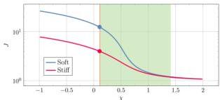Fig. 4 Swelling ratio $J$ versus Flory parameter $\chi$ for the stiff $(G = 6.79 \times 10^{6} \, \mathrm{Pa})$ and the soft $(G = 8.67 \times 10^{5} \, \mathrm{Pa})$ material. The temperature dependent $\chi_{\mathrm{eff}}$ ranges in the green shadowed area; two circles on the vertical line at $\chi = 0.2$ show the initial values $J_{\mathrm{soil}} = 1 / \phi_{\mathrm{oi}}$ of the swelling ratio.

This journal is © The Royal Society of Chemistry 2026

Soft Matter, 2026, 22, 3238-3251

---

Soft Matter

Paper

temperature; the two circles on the vertical line $\chi = 0.2$ indicate the initial swelling state of each domain. This figure illustrates how the thermally induced shift in $\chi_{\mathrm{eff}}$ drives differential deswelling between the two domains.

We study thermal dehydration for two bilayer geometries: a disk with a base diameter of $L$ and height $H$ ; a square prism with a base of side length $L$ and height $H$ . Both geometries have horizontal base in the plane $\mathbf{e}1, \mathbf{e}_2$ and height aligned with $\mathbf{e}_3$ ; moreover, both geometries have a stiff top layer with thickness $H{\mathrm{T}} = \alpha H$ and a soft bottom layer with thickness $H_{\mathrm{B}} = (1 - \alpha)H$ .

We note that the parameters $\mu_0, \phi_{oi} G_i$ and $\chi_{\mathrm{eff}}$ are interdependent. We consider two different pairs $(\phi_{o1}, \phi_{o2})$ of initial solid fractions, yielding two different values of the ratio $G_2 / G_1$ ; the values of $\phi_{oi}$ , of the shear moduli $G_i$ , the initial values of the Flory parameter $\chi_{oi} = \chi_{\mathrm{eff}}(T_o, \phi_{oi})$ , and of the variables $c_{oi}, p_{oi}$ are given in Table 2.

Finally, we study dehydration under different external temperatures $T_{\mathrm{ext}} = T_0 + \Delta T$ , with temperature gradient $\Delta T = 0, 20, 40, 60 \mathrm{~K}$ ; for $\Delta T = 0 \mathrm{~K}$ , dehydration is driven solely by the relative humidity gradient. Given the value of Tables 1 and 2, eqn (68) predicts the following pairs $(T_{\mathrm{ext}}, T_{\mathrm{wb}})$ for the four temperature gradients $\Delta T$

(293 K, 289 K), (313 K, 305 K), (333 K, 322 K), (353 K, 338 K). (69)

Note, for the condition of $\Delta T = 60\mathrm{K}$ , both the wet-bulb temperature $T_{\mathrm{wb}}$ and external temperature $T_{\mathrm{ext}}$ exceed the denaturation temperature $T_{\mathrm{d}} = 323\mathrm{K}$ . Hence, first shrinkage will occur already in the initial heating stage due to protein denaturation. As denaturation happens over a broad temperature range, we wonder if this is can be distinguished from regular dehydration shrinkage happening in the CDR regime. For $\Delta T = 40\mathrm{K}$ , $T_{\mathrm{wb}} \approx T_{\mathrm{d}} < T_{\mathrm{ext}}$ , the two stages of shrinkage will definitely overlap.

Our analysis centers on three main topics: (1) the mechanical response of the system, including its propensity for shape changes such as bending and wrinkling, as well as the accumulation of stress. (2) The mass transport, investigating how water moves across internal interfaces and through external boundaries. (3) The thermodynamic effects, differentiating between heat transfer driven by convection and heat transfer due to water evaporation.

Table 2 Parameters used for bilayers with high and low ratio ${G}{2}/{G}{1}$

High G2/G1= 7.09	Low G2/G1= 4.48	Units
φo1= 0.0933	φo1= 0.3375	1
φo2= 0.2800	φo2= 0.6293	1
χeff(T0)= 0.2	Initial χeff for soft	1
χeff(T0)= 0.25	Initial χeff for stiff	1
co1= 50	co1= 37	kmol m-3
co2= 40	co2= 21	kmol m-3
po1= 3.87 × 105	po1= 6.96 × 106	Pa
po2= 3.94 × 106	po2= 3.84 × 107	Pa
G1= 8.53 × 105	G1= 1.00 × 107	Pa
G2= 6.02 × 106	G1= 4.48 × 107	Pa

Furthermore, a key focus is identifying the stage of the drying process in which shape morphing (i.e., differential shrinkage) is most pronounced. We frame this analysis using the four classic drying phases: (a) the preheating period; (b) the CDR period, characterized by the wet-bulb temperature; (c) the falling rate period; (d) the approach to equilibrium.

Let $V_{\mathrm{si}}$ be the dry volume and $V_{\mathrm{wi}}$ the initial water volume of domain $i$ ; the ratio $V_{\mathrm{wi}} / V_{\mathrm{si}}$ is given by the formula

\[\frac {1}{\phi_ {o i}} = J _ {e o i} = \frac {V _ {\mathrm {s}} + V _ {\mathrm {w i}}}{V _ {\mathrm {s}}} \Rightarrow \frac {V _ {\mathrm {w i}}}{V _ {\mathrm {s}}} = J _ {e o i} - 1. \tag {70}\]

From the initial solid fractions of Table 2, we have $V_{\mathrm{w1}} / V_{\mathrm{s1}} = 9.71$ and $V_{\mathrm{w2}} / V_{\mathrm{s2}} = 2.57$ for high ratio $G_{2} / G_{1}$ , and $V_{\mathrm{w1}} / V_{\mathrm{s1}} = 2.96$ and $V_{\mathrm{w2}} / V_{\mathrm{s2}} = 0.59$ for low ratio $G_{2} / G_{1}$ . Based on the results of our model, we can evaluate several important integral quantities. Specifically, we calculated the average heat power source at the boundary $(\mathrm{Wm}^{-2})$ , telling between the total heat $Q_{\mathrm{hi}}$ and the heat power due to water evaporation $Q_{\mathrm{hwi}}$ :

\[Q _ {\mathrm {h i}} (t) = \frac {1}{A _ {i}} \int_ {\partial \mathcal {B} _ {\mathrm {e x t}, i}} s _ {\mathrm {h i}} (x, t) \mathrm {d} A, \tag {71}\] \[Q _ {\mathrm {h w i}} (t) = \frac {1}{A _ {i}} \int_ {\partial \mathcal {B} _ {\mathrm {e x t}, i}} s _ {\mathrm {h w i}} (x, t) \mathrm {d} A;\]

moreover, we calculated the water exchange $W(t)$ at time $t$ by

\[W (t) = \Omega \int_ {0} ^ {t} \left(Q _ {\mathrm {w} 1} (\tau) + Q _ {\mathrm {w} 2} (\tau)\right) \mathrm {d} \tau \quad [ W ] = \mathrm {m} ^ {3}, \tag {72}\]

where $Q_{\mathrm{wi}}(t)$ is the water source at the boundary $\partial \mathcal{B}_{\mathrm{ext},i}$ , given by

\[Q _ {\mathrm {w i}} (t) = \int_ {\partial \mathcal {B} _ {\mathrm {e x t}, i}} s _ {\mathrm {w i}} (x, t) \mathrm {d} A, \quad [ Q _ {\mathrm {w i}} ] = \operatorname {m o l} \left(\mathrm {m} ^ {- 2} \mathrm {s} ^ {- 1}\right). \tag {73}\]

The quantities $s_{\mathrm{hi}}, s_{\mathrm{hwi}}, s_{\mathrm{wi}}$ are given by (31), (51), (52) and (54), while the area $A_{i}$ of $\partial \mathcal{B}_{\mathrm{ext},i}$ is evaluated by

\[A _ {i} = \int_ {\partial \mathcal {B} _ {\mathrm {e x t}, i}} 1 \mathrm {d} A. \tag {74}\]

4 Results

Through our modeling, it is possible to follow the time evolution of the three state variables displacement, water content and temperature during dehydration. Our system reveals distinct dehydration dynamics within the two domains. From a mechanical perspective, this differential drying induces frustration and stress, ultimately causing the material to bend and possibly wrinkle.

From a thermodynamic standpoint, this system exhibits a key feature known as the wet-bulb effect: the evaporation of water absorbs a significant amount of heat. This phenomenon allows the average temperature to remain remarkably stable over an extended period.

In the preheating stage, the specimen quickly rises from its initial temperature to the wet-bulb temperature. The time scale of this stage is governed by both external and internal heat transfer mechanisms. During the CDR period, both the

Soft Matter, 2026, 22, 3238-3251

This journal is © The Royal Society of Chemistry 2026

---

Paper

Soft Matter

temperature and the drying rate $\mathrm{d}J / \mathrm{d}t$ may remain constant because all the incoming heat power is consumed by the evaporation of water: $s_{\mathrm{h}} = s_{\mathrm{hc}} + s_{\mathrm{hw}} = 0$ .

When drying starts, $a_{\mathrm{w}} \approx 1$ ; the CDR ends when the water activity deviates significantly from unity $a_{\mathrm{w}} < 0.95$ . The moisture sorption isotherm is assumed to follow Flory-Huggins theory; via this isotherm it is possible to compute the corresponding moisture content.

The latent heat of evaporation (55) is always positive. Therefore, considering the expressions for the water source (31) and the heat source due to evaporation (54), it follows that

\[\begin{array}{l} \Delta c _ {\mathrm {v}} = c _ {\mathrm {v}, \text {e x t}} \left(T _ {\text {e x t}}\right) - c _ {\mathrm {v}} (T) \leq 0 \quad \Rightarrow \quad s _ {\mathrm {w}} \leq 0 \quad \Rightarrow \tag {75} \\ s _ {\mathrm {h w}} \leq 0 \\ \end{array}\]

Thus, the sign of $\Delta c_{\mathrm{v}}$ determines whether water enters or leaves the specimen. The associated heat power source corresponds directly to this process, sharing the same sign as the mass source term. From (23) and (25), and given the values listed in Table 1, the initial difference in temperature $T_{\mathrm{ext}} - T_{\mathrm{o}}$ has an important role. For moderate heating, $\Delta c_{\mathrm{v}}$ remains always negative, for more intense heating, $\Delta c_{\mathrm{v}}$ is initially positive and water enters the specimen.

For a wet hydrogel like (Sephadex) dextran gel of grade G50 (with elastic modulus in order of $G = 10 \, \mathrm{kPa}$ ) the polymer volume fraction can decrease a factor of 10 in this range.[26,44] Note that the wet-bulb temperature is independent of material properties of the food, but it is only defined by the drying conditions.

For drying of bilayer specimen, composed of a soft and stiff food-like material, we expect most of the morphing to happen in the CDR period, while the falling rate period has the only function of stabilizing the formed shape (via bringing to the glassy state, and lower its water activity to levels required for microbial safety ( $a_{\mathrm{w}} < 0.6$ ). To quantify the change of shape with respect to the initial flat configuration, we evaluate the curvatures $k_{x}$ and $k_{y}$ of a horizontal cross-section along the $x$ and $y$ directions, calculated using the formula:

\[k _ {x} = \frac {w _ {x x} \left(1 + u _ {x}\right) - w _ {x} u _ {x x}}{\left(\left(1 + u _ {x}\right) ^ {2} + w _ {x} ^ {2}\right) ^ {3 / 2}} \quad k _ {y} = \frac {w _ {y y} \left(1 + v _ {y}\right) - w _ {y} u _ {y y}}{\left(\left(1 + v _ {y}\right) ^ {2} + w _ {y} ^ {2}\right) ^ {3 / 2}}. \tag {76}\]

4.1 Disk geometry

We report the main findings for the disk geometry with $\mathrm{ar} = 8$ , 20, and $\alpha = 0.5$ . Fig. 5 shows some configurations realized during the drying at $\Delta T = 60 \mathrm{~K}$ ; the left panel displays a vertical cross-section of a disk, comparing its initial swollen state (top) with the final dry state (bottom). The lower image represents the hypothetical outcome of the two distinct domains dehydrating in isolation. The right panel illustrates the time evolution of the disk configuration for the case $\Delta T = 60 \mathrm{~K}$ , colored with the polymer fraction. The top row displays configurations at early stages of the process, while the bottom row shows later stages.

It is worth noting the evolution of curvature—from initially flat, to concave in the early stages, and eventually to convex.

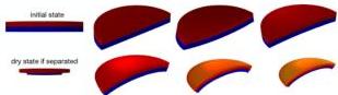Fig. 5 Disk dehydration. Left: vertical cross section of initial swollen state (top) and final dry state if separated (bottom). Right: configurations at $t = 0$ s, $2 \times 10^{2}$ s, $10^{3}$ s (top) and $t = 2 \times 10^{3}$ s, $5 \times 10^{3}$ s, $10 \times 10^{3}$ s (bottom). Aspect ratio $= 8$ , $\alpha = 0.5$ . Colors represent the magnitude of the polymer fraction $\phi$ , ranging from blue (minimum, corresponding to the fully swollen initial state) to red (maximum, corresponding to the dry state).

The temporary concave shape arises from the initial water uptake predicted by eqn (75) under intense heating and high humidity.

The wet-bulb effect can be analyzed with the next two figures.

Fig. 6 consists of two panels, both plotted against time on a logarithmic scale. The left panel shows the average swelling ratio $(J,$ left $y$ -axis) and the average surface temperature $(T,$ right $y$ -axis); the right panel shows the average swelling rate $(\mathrm{d}J / \mathrm{d}t,$ left $y$ -axis) and the average surface temperature $(T,$ right $y$ -axis). Note: All averages $(J,T,$ and $\mathrm{d}J / \mathrm{d}t)$ are calculated over either the whole disk or the disk boundary. The wet-bulb effect produces a plateau in the temperature plot; as example, for $\Delta T = 60~\mathrm{K}$ , the CDR time interval starts at $t_1\simeq 200$ s and ends at $t_2\simeq 6000$ s. It is during this time interval that the swelling $J$ decreases significantly, while swelling rate $\mathrm{d}J / \mathrm{d}t$ has the largest negative value, corresponding to water release. This effect holds for any $\Delta T$ ; for $T_{\mathrm{ext}} = T_{\mathrm{o}}$ , drying is only due to relative humidity, and during the CDR time interval, the average temperature is lower than the ambient one.

Fig. 7 displays two sets of time-dependent (log scale) results. The left panel presents the surface-averaged total heat source $(Q_{\mathrm{h}},$ left axis) and the temperature $(T,$ right axis), for four

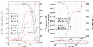Fig. 6 Disk dehydration dynamics. Left: average swelling ratio $J$ (left $y$ -axis, solid colored) and average temperature $T$ (right $y$ -axis, dashed red) versus time (log scale), with $\Delta T = 0, 20, 40, 60 \mathrm{~K}$ . Right: average drying rate $\mathrm{d}J / \mathrm{d}t$ (left $y$ -axis, solid black) and average temperature $T$ (right $y$ -axis, dashed red) versus time (log scale), with $\Delta T = 0, 60 \mathrm{~K}$ . Dot-dashed curves show reference values: red for $T_{\mathrm{ext}}$ ; black for $J = 1$ and $\mathrm{d}J / \mathrm{d}t = 0$ . For $\Delta T = 60 \mathrm{~K}$ , the wet-bulb effect occurs in the time interval from $t_1 \simeq 200$ s to $t_2 \simeq 7000$ s, during which swelling $J$ decreases significantly (left plot), while swelling rate $\mathrm{d}J / \mathrm{d}t$ has its lowest value (right plot). Aspect ratio $= 8$ , $\alpha = 0.5$ .

This journal is © The Royal Society of Chemistry 2026

Soft Matter, 2026, 22, 3238-3251

---

Soft Matter

Paper

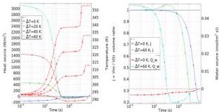Fig. 7 Disk dehydration dynamics. Left: average heat source $Q_{\mathrm{n}}$ (left y-axis, solid colored lines) and average temperature $T$ (right y-axis, dashed red lines) versus time (log scale). Right: average swelling ratio $J$ (left y-axis, solid colored) and average water source $s_{\mathrm{w}}$ (right y-axis, dashed colored) versus time (log scale). Curves corresponding to the same temperature share the same marker type.

distinct temperature differences $\Delta T$ . The right panel presents the swelling ratio $(J,$ left axis) and the surface-averaged water source $(Q_{\mathrm{w}},$ right axis), only for the cases $\Delta T = 0$ $60~\mathrm{K}$

For $\Delta T \geq 20\mathrm{K}$ , the heat source terms is initially positive over a short time interval, indicating that the specimen is heating up and water is entering. When $Q_{\mathrm{h}} \simeq 0$ , the wet-bulb effect starts, the temperature remains almost constant for a long time interval, and water begins to leave the specimen. Eventually, the heat and water sources approach zero and the system reaches thermo-chemical equilibrium. For $\Delta T = 0\mathrm{K}$ , both the heat and water source terms remain negative throughout the process. In this case, the specimen temperature stays below the external temperature for an extended period.

Fig. 8 shows a domain-wise analysis of the dehydration dynamics for $\Delta T = 60\mathrm{K}$ . In both panels, we also include averages evaluated separately on each domain. Left panel shows the average heat source at the boundary $Q_{\mathrm{hi}}$ on the left $y$ -axis, and average temperature $T_{i}$ on the right $y$ -axis, versus time (log scale). The right panel shows the average swelling ratio $J$ on the left $y$ -axis, and average water source $Q_{\mathrm{wi}}$ on the right $y$ -axis, versus time (log scale). Both heating power and the

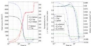Fig. 8 Domain-wise dehydration dynamics for $\Delta T = 60\mathrm{K}$ . Left: average heat source at the boundary $Q_{\mathrm{hi}}$ on the left $y$ -axis, and average temperature $T_{i}$ on the right $y$ -axis, are plotted against time (log scale). Right: average swelling ratio $J$ on the left $y$ -axis, and average water source $Q_{\mathrm{wi}}$ on the right $y$ -axis, versus time (log scale). Aspect ratio $= 8$ , $\alpha = 0.5$ ; average evaluated separately on each domain.

water source flux are higher in the soft bottom domain compared to the stiff top domain. The initial volume increase is attributed to water uptake in the soft domain, while temperatures remain very similar across both domains. This water uptake produces the concave configuration observed at early stages, as shown in Fig. 5.

The duration $\tau_{\mathrm{CDR}}$ of the CDR can be obtained from the difference in moisture content divided by the drying rate; with reference to Fig. 8, we have $\tau_{\mathrm{CDR}} \sim (1 - 0.2) / 10^{-4} \sim 8 \times 10^{3} \mathrm{~s}$ .

In the falling rate period, the internal moisture transport becomes rate limiting, as the moisture diffusion coefficient will decrease over several decades if the material goes from the rubbery regime to the glassy state.[45] For sufficient large food products the surface will form a (glassy) crust, and its diffusion coefficient with the moisture gradient will determine the falling drying rate. Nevertheless, in our model we assume a constant diffusion coefficient, and the falling rate period is shorter than the CDR period.

The disk geometry characterized by an aspect ratio $\alpha = 20$ and $\alpha = 0.5$ initially exhibits a dome-like shape, similar to the $\alpha = 8$ case. However, this shape eventually buckles, transitioning into a configuration featuring distinct lobes. For this specific geometry ( $\alpha = 20$ , $\alpha = 0.5$ ), we conduct an investigation into the complex evolution of curvature and water content versus average temperature and time. Fig. 9 presents the coupled dehydration dynamics using two separate plots. Both the top and bottom plots display the curvature $(\mathrm{m}^{-1})$ on the left $y$ -axis and the volume of expelled water $(\mathrm{mm}^3)$ on the right $y$ -axis.

The left plot shows the evolution with respect to temperature (K), while the right plot shows the evolution with respect to time (s). The six illustrative configurations shown below the plots correspond to the red data points marked in the figures

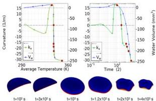Fig. 9 Disk dehydration dynamics: coupled curvature and water expulsion dynamics. In both figures, the curvature $(\mathrm{m}^{-1})$ and the volume of expelled water $(\mathrm{mm}^3)$ are presented on the left and right $y$ -axes, respectively. The left plot shows the evolution with respect to temperature (K), while the right plot shows the evolution with respect to time (log scale). The six configurations below correspond to the red data points in the plots. Crucially, the major change in shape (curvature) is observed during the time interval where the temperature remains stable. Aspect ratio = 20, $\alpha = 0.5$ .

Soft Matter, 2026, 22, 3238-3251

This journal is © The Royal Society of Chemistry 2026

---

Paper

Soft Matter

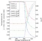
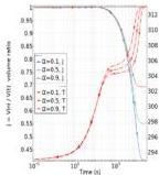Fig. 10 Prism. Influence of $\alpha$ on dehydration dynamics. Left: average swelling $J$ (left $y$ -axis) and average temperature $T$ (right $y$ -axis) versus time (log scale). Right: average swelling $J$ (left $y$ -axis) and average effective Flory-Huggins $\chi_{\mathrm{eff}}$ (right $y$ -axis) versus temperature. For both panels, $\alpha = 8$ and $\alpha = 0.1, 0.5, 0.9$ .

above. Note that the most significant shape change (indicated by the change in curvature) occurs during the interval where the average temperature remains nearly constant; in particular, buckling from dome-like to lobes appears at $t \simeq 10^3$ , and $T \simeq 340 \mathrm{~K}$ .

4.2 Prism geometry

For the prism geometry, we analyze a thick specimen $(\mathrm{ar} = 8)$ and a thin one $(\mathrm{ar} = 20)$ ; for both aspect ratios, we study the effect of $\alpha$ in the range $\alpha = (0.1, 0.9)$ , with step 0.1; we solve for mild heating, that is $\Delta T = 20 \mathrm{~K}$ .

Fig. 10 illustrates the significant influence of the parameter $\alpha$ on the dehydration dynamics of a prism with an aspect ratio of $\mathrm{ar} = 8$ . The results for three distinct $\alpha$ values ( $\alpha = 0.1, 0.5$ , and 0.9) are presented. The left panel shows the average swelling $J$ (left $y$ -axis) and the average temperature $T$ (right $y$ -axis) versus time (log scale). It is worth highlighting the constant drying rate (CDR) regimes, where the measured wet-bulb temperatures range between $304\mathrm{K}$ and $306\mathrm{K}$ . This experimental range is in excellent agreement with the theoretical prediction of $T_{\mathrm{wb}} = 305\mathrm{K}$ , calculated using eqn (68). The right panel shows the average swelling $J$ (left $y$ -axis) and the average effective Flory-Huggins $\chi_{\mathrm{eff}}$ (right $y$ -axis) versus temperature; significant volume contraction is concentrated within a small interval of temperature change.

Fig. 11 and 12 show the final configurations after dehydration for $\mathrm{ar} = 8$ and $\mathrm{ar} = 20$ , respectively, upon mild heating $T_{\mathrm{ext}} = T_{\mathrm{o}} + 20\mathrm{K}$ . The main result shows the existence of a threshold for $\alpha$ , below which the final shape develops four distinct lobes at the corners.

4.3 Effects of Flory parameter

Finally, we investigate the influence of the Flory parameter on dehydration dynamics by addressing the same physical problem through three distinct formulations for $\chi$ : (i) $\chi_{\mathrm{eff}}$ , which depends on both temperature and solid fraction as defined in eqn (18); (ii) $\chi_{\phi}$ , which depends exclusively on the solid fraction $\phi$ via $\chi_{\phi} = \chi_{0} + (\chi_{\infty} - \chi_{0})\phi^{2}$ ; and (iii) a constant value $\chi_{0}$ . Our results indicate that while shape evolution is highly sensitive to

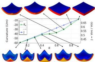Fig. 11 Prism dehydration. Influence of $\alpha$ on the final configurations for ar $= 8$ . The plot shows the curvature, $k_{x}$ , measured at the center of the geometry (left y-axis), and the swelling ratio (right y-axis) versus $\alpha$ . The shape is always a dome in the full range $0.1 \leq \alpha \leq 0.9$ .

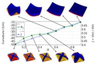Fig. 12 Prism dehydration. Influence of $\alpha$ on the final configurations for $\mathrm{ar} = 20$ . The plot shows the curvature, $k_{x}$ , measured at the center of the geometry (left y-axis), and the swelling ratio (right y-axis) versus $\alpha$ . The results reveal a transition in the final configuration: for $\alpha \geq 0.4$ , the shape is a dome, whereas for $\alpha \leq 0.5$ , the shape develops four distinct lobes at the corners $\mathrm{ar} = 20$ .

the specific choice of $\chi$ , the water exchange and wet-bulb temperature remain largely unaffected. For brevity, we report results exclusively for the disk geometry with $\mathrm{ar} = 8$ and $\alpha = 0.5$ . Fig. 13 illustrates the curvature $k_{x}$ at the top center of the disk and the volume of water exchanged $W$ , calculated via eqn (72), as functions of time (left panel) and temperature (right panel).

We note that water volume plots (blue lines) are almost superimposed for the three cases; conversely, curvature plot (green lines) are quite different.

5 Discussion

Our principal results concern the role of differential dehydration rates observed between the two domains, and the role of water evaporation in the heating power exchanged at the boundary.

This journal is © The Royal Society of Chemistry 2026

Soft Matter, 2026, 22, 3238-3251

---

Soft Matter

Paper

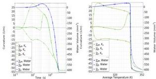Fig. 13 Disk. Influence of Flory parameter on dehydration dynamics. Left: curvature $k_{x}$ (left $y$ -axis) and water volume $W$ (right $y$ -axis) versus time (log scale). Right: curvature $k_{x}$ (left $y$ -axis) and water volume $W$ (right $y$ -axis) versus temperature. For both panels, $\alpha = 8$ and $\alpha = 0.5$ .

The differential dehydration rate is the direct result of the coupled thermo-hydro-mechanical equations. Specifically, the varying elastic modulus $(G)$ and Flory parameter $(\chi)$ between the domains, combined with the non-uniform water concentration $(c_{i})$ across the interface, drives the imbalance.

Differential dehydration directly generates localized stresses and domain-specific shrinkage: the faster-shrinking domain imposes a mechanical constraint on the slower-shrinking domain. This mismatched deformation creates internal stresses, similar to thermal stresses, but driven by both moisture content and differential elastic stiffness. The build-up of such a stress is responsible for the overall shape morphing or potential cracking/delamination of the material.

The second important feature is the prediction of a critical temperature thresholds and the wet-bulb effect. This effect, where the surface temperature remains lower than the ambient temperature due to evaporative cooling, demonstrates that the process is kinetically limited by heat transfer early on. The critical temperature threshold marks the point where the drying mechanism transitions from constant-rate drying (heat-transfer limited) to falling-rate drying (moisture-diffusion limited).

The multiphysics model herein presented successfully captures this phase transition, which is often simplified or ignored in purely mechanical or purely diffusion-based models.

Our mechanical modeling draws heavily on poroelastic concepts, and hydrogel swelling, but is augmented by incorporating thermal effects and large volume changes due to dehydration. In particular, the large deformation theory developed for swelling is robustly applied to the case of thermal shrinkage.

Our work is connected to established models in food science and industrial drying, $^{13,14,24,25}$ and is able to capture the observed drying curves (mass loss vs. time/temp), likewise the constant-rate and falling-rate periods.

Our main contribution over these models is the mechanical feedback. Food drying models often neglect the resulting internal stresses and geometry changes that your model captures, which are crucial for the structural integrity of soft materials.

Our localized stress findings support the body of work on mechanical instabilities and shape morphing in bi-layered/bi-domain soft materials. The dehydration process provides a

precise, thermally-controlled way to trigger these instabilities (e.g., curling, buckling). The properties of the domain interface dictate the type and scale of the mechanical instability. A weak interface might lead to delamination, while a strong one might lead to severe buckling.

6 Conclusions

This study provides a comprehensive model for dehydration in bi-domain soft materials under temperature variations. The results underscore the importance of domain interfaces and material properties in controlling the thermo-hydro-mechanical response. These findings pave the way for designing advanced soft materials with tailored dehydration characteristics.

Our findings have practical relevance for future modeling and research. The results provide a blueprint for designing thermally responsive soft materials with tailored shrinkage profiles. By tuning the $G_{1} / G_{2}$ ratios or thermal properties of the two domains, it is possible to predict and control the final shape or stability. This conclusion is drawn directly from our parametric simulations, where varying the stiffness ratio $G_{1} / G_{2}$ dictates the relative extent of shrinkage between the core and the skin. A larger mismatch exacerbates the differential strain at the interface, driving the structure to buckle or bend to minimize total elastic energy, thereby controlling the final morphing geometry.

The identified critical temperature thresholds are vital for industrial or biomedical applications (e.g., drug delivery). Understanding these limits allows for efficient drying without inducing failure (cracking or excessive residual stress).

It is worth acknowledging the model limitations; we cite the assumption of ideal gas behavior for the evaporated moisture, the material isotropy maintained throughout the dehydration process, the non-linear dependencies of diffusion $D$ on moisture content.

Future work includes experimental validation focused on the predicted stress fields or morphological changes, and the incorporation of additional factors, such as porosity collapse (irreversible shrinkage) or chemical reactions (e.g., heat-induced curing) to model more complex, real-world materials.

Conflicts of interest

There are no conflicts to declare.

Data availability

All numerical experiments presented in the manuscript entitled “Thermal dehydration of swollen heterogeneous soft materials insert title” for possible publication on Soft Matter were performed using COMSOL Multiphysics. The COMSOL models used in this study are available from the authors upon reasonable request and can be used to reproduce the results and data presented in this work.

Soft Matter, 2026, 22, 3238-3251

This journal is © The Royal Society of Chemistry 2026

---

Paper

Soft Matter

Acknowledgements

We gratefully acknowledge the support by the Italian Ministry of Research through the project Innovative mathematical models for soft matter and hierarchical materials (PRIN 2022, PNRR F53D2300283 0006). The authors LT and GT are member of the INdAM GNFM research group.

Notes and references

1. J. Li and D. J. Mooney, Nat. Rev. Mater., 2020, 11, 256-265.
2. P. Calvert, Adv. Mater., 2009, 21, 743-756.
3. M. A. C. Stuart, W. T. Huck, J. Genzer, M. Müller, C. Ober, M. Stamm, G. B. Sukhorukov, I. Szleifer, V. V. Tsukruk and M. Urban, et al., Nat. Mater., 2010, 9, 101-113.
4. Y. Zhang, et al., Mater. Today, 2023, 42, 100-115.
5. D. Floreano, B. Kwak, M. Pankhurst, J. Shintake, M. Caironi, V. F. Annese, Q. Qi, J. Rossiter and R. M. Boom, Nat. Rev. Mater., 2024, 9, 589-599.
6. R. van der Sman, M. Curatolo and L. Teresi, Curr. Res. Food Sci., 2025, 10, 101074.
7. V. Rakesh and A. K. Datta, AIChE J., 2013, 59, 33-45.
8. T. Gulati and A. K. Datta, Chem. Eng. Sci., 2016, 139, 75-98.
9. K. Seranthian and A. Datta, Chem. Eng. Sci., 2023, 277, 118802.
10. W. Hong, X. Zhao, J. Zhou and Z. Suo, J. Mech. Phys. Solids, 2008, 56, 1779-1793.
11. S. Cai and Z. Suo, J. Mech. Phys. Solids, 2011, 59, 2259-2278.
12. M. Curatolo, R. G. M. van der Sman and L. Teresi, J. Elasticity, 2024, 156, 1195-1241.
13. R. Van der Sman, AIChE J., 2007, 53, 2986-2995.
14. R. van der Sman, M. Curatolo and L. Teresi, Curr. Res. Food Sci., 2024, 8, 100762.
15. X. Jin and R. van der Sman, Food Struct., 2022, 32, 100269.
16. R. van der Sman, M. Curatolo and L. Teresi, Soft Matter, 2024, 20, 5183-5194.
17. R. van der Sman, M. Curatolo and L. Teresi, Curr. Res. Food Sci., 2025, 11, 101238.
18. J. Grasa, L. Teresi and R. van der Sman, Curr. Res. Food Sci., 2025, 101230.
19. A. Lucantonio, P. Nardinocchi and L. Teresi, J. Mech. Phys. Solids, 2013, 61, 205-218.
20. A. Stracuzzi, E. Mazza and A. E. Ehret, Z. Angew. Math. Mech., 2018, 98, 2135-2154.
21. Y. Dadmohammadi and A. K. Datta, Food Rev. Int., 2022, 38, 953-985.
22. Y. Shi and T. Wallmersperger, J. Intell. Mater. Syst. Struct., 2022, 1045389X221093347.
23. D. Caccavo, G. Lamberti and A. A. Barba, Eur. J. Pharm. Biopharm., 2020, 152, 299-306.
24. J. Moya, S. Lorente-Bailo, M. Salvador, A. Ferrer-Mairal, M. Martinez, B. Calvo and J. Grasa, J. Food Eng., 2021, 298, 110498.
25. A. Dhall and A. K. Datta, Chem. Eng. Sci., 2011, 66, 6482-6497.
26. R. Brighenti and M. P. Cosma, J. Mech. Phys. Solids, 2022, 169, 105045.
27. S. A. Chester and L. Anand, J. Mech. Phys. Solids, 2011, 59, 1978-2006.
28. R. Van der Sman, Food Hydrocolloids, 2015, 48, 94-101.
29. M. Curatolo, P. Nardinocchi, E. Puntel and L. Teresi, J. Appl. Phys., 2017, 122, 145109.
30. M. Shojaeifard, S. Niroumandi and M. Baghani, Acta Mech., 2022, 233, 213-232.
31. M. B. Amar and A. Goriely, J. Mech. Phys. Solids, 2005, 53, 2284-2319.
32. M. B. Amar and P. Ciarletta, J. Mech. Phys. Solids, 2010, 58, 935-954.
33. M. Curatolo, P. Nardinocchi, E. Puntel and L. Teresi, J. Appl. Phys., 2017, 122, 145109.
34. Y. Zhang, O. Y. Cohen, M. Moshe and E. Sharon, Science, 2025, 388, 520-524.
35. P. Nardinocchi, L. Teresi and D. P. Holmes, Mechanics of Swelling, Royal Society of Chemistry, 2026.
36. R. Van der Sman, Food Hydrocolloids, 2012, 27, 529-535.
37. R. Van der Sman and M. Meinders, Soft Matter, 2011, 7, 429-442.
38. A. K. Datta, Biological and Bioenvironmental Heat and Mass Transfer, Marcel Dekker, New York, 2002.
39. R. B. Bird, W. E. Stewart and E. N. Lightfoot, Transport Phenomena, John Wiley & Sons, New York, Revised 2nd edn, 2006.
40. A. K. Datta, J. Food Eng., 2007, 80, 96-110.
41. A. K. Datta, J. Food Eng., 2007, 80, 80-95.
42. S. J. Kowalski, Thermomechanics of Drying Processes, Springer, Berlin, Heidelberg, 2003, vol. 8.
43. Handbook of Industrial Drying, ed. A. S. Mujumdar, CRC Press, Boca Raton, FL, 4th edn, 2015.
44. R. Van Der Sman, Food Funct., 2018, 9, 2716-2724.
45. R. Van der Sman and M. Meinders, Food Chem., 2013, 138, 1265-1274.

This journal is © The Royal Society of Chemistry 2026

Soft Matter, 2026, 22, 3238-3251