Surface growth

For the pdf version of this page click here

1 Treadmilling

The algebraic-differential system.

After working out the equations (we refer to the manuscript for details), we arrive at a system of differential algebraic equations which can be conveniently written in the form

	$\dot{\mathrm{\ell }}$	$=R_1(\sigma )-R_0(\sigma )$
	$\mathrm{\ell }$	$=\widehat{\mathrm{\ell }}(\sigma ).$

The unknowns the reference length $\mathrm{\ell }$ and the traction $\sigma$.

Treadmilling solutions

We are interested in stationary solutions of (1). These are called “treadmilling solutions”, since they replicate the treadmilling mechanism of actin growth. Finding such solutions is equivalent to solving

$$R_0(\sigma )=R_1(\sigma ).$$

(1)

To this effect, the form of $\widehat{\mathrm{\ell }}(\sigma )$ is irrelevant (it becomes relevant when we are to assess stability).

The accretion rates $R_0(\sigma )$, $R_1(\sigma )$.

The functions in (1) are defined as follows

		$R_1(\sigma )={\displaystyle \frac{1}{B_1}}\left(W^{*}(\sigma )-W^{*}({\sigma }_{B1})\right)$		(2)
		$R_0(\sigma )=-{\displaystyle \frac{1}{B_0}}{\displaystyle \frac{{\sigma }_{\mathrm{asym}}-{\sigma }_{\max }}{{\sigma }_{\mathrm{asym}}-\sigma }}\left(W^{*}(\sigma )-W^{*}({\sigma }_{B0})\right)$
		$\widehat{\mathrm{\ell }}(\sigma )={\displaystyle \frac{{\sigma }_{\max }-\sigma }{K{W}^{*}{}^{\prime }(\sigma )}}.$

The accretion rates $R_0$ and $R_1$, which are our major concern, depend on four parameters: ${\sigma }_{B0}$, ${\sigma }_{B1}$, ${\sigma }_{\max }$ and ${\sigma }_{\mathrm{asym}}$. As the symbols suggests, all of these quantities have physical dimension of a force (traction).

Blocking tractions.

The blocking tractions ${\sigma }_{B0}$ and ${\sigma }_{B1}$ are defined by

$$W^{*}({\sigma }_{B0})+\varrho ({\mu }_1-{\mu }_{B0})=0,W^{*}({\sigma }_{B1})+\varrho ({\mu }_1-{\mu }_{B1})=0.$$

(3)

Comparing these expressions with the expressions for the driving forces, we see that these are the stresses that should be applied at each end of the bar to stop its growth if the chemical potential was everywhere equal to ${\mu }_1$ (this would be the case if the mobility of the diffusant was infinite).

The maximal traction and the asymptotic traction.

Two other parameters that define $R_0$ and $R_1$ are the maximal traction and the asymptotic traction, defined respectively by

$${\sigma }_{\max }=K(Y_1-Y_0)\mathit{\hspace{1em}\hspace{1em}}\text{and}\mathit{\hspace{1em}\hspace{1em}}{\sigma }_{\mathrm{asym}}={\sigma }_{\max }+\frac{m{B}_{0}K}{{\varrho }^2}.$$

(4)

The stress ${\sigma }_{\max }$ is the traction produced by the spring when the extreme points of the bar collapse on the clamped end. Would the spring be stretched beyond that point, the stretch $\lambda$ in the bar would be negative, a situation that is prevented by the blowup of the strain energy as $\lambda$ approaches zero from the positive side.

Properties of the functions $R_0$ and $R_1$.

The properties of $R_0$ and $R_1$ are discussed extensively in [1]. For our purposes, it suffices to use a few plots.

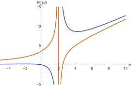
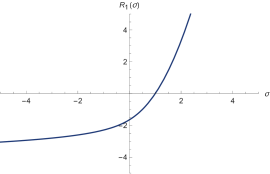
Here, on the left, we show the plot of $R_0$ for (blue) and ${\sigma }_{B0}>{\sigma }_{\mathrm{asym}}$ (orange). On the right, we show the plot of $R_1(\sigma )$. The important properties of $R_0$ and $R_1$ are the following:

• $R_0$ and $R_1$ vanish at the corresponding blocking stresses.

• $R_1$ is a monotone increasing convex function which tends to $\pm \mathrm{\infty }$ as $\sigma \to \pm \mathrm{\infty }$.

• the behavior of $R_0$ is more complicated that than of $R_1$, because $R_0$ is affected by the kinetic of diffusion throug the parameter ${\sigma }_{\mathrm{asym}}$. In particular, $R_0$ has a singularity at ${\sigma }_{\mathrm{asym}}$, and its shape depends crucially on the relative value of ${\sigma }_{B0}$ and ${\sigma }_{\mathrm{asym}}$.

Treadmilling solutions.

To understand under what circumstances treadmilling solutions are possible, it is useful to consider different cases and draw some illustrating plots. In drawing these plots we have shifted the origin of $\sigma$ so that the vertical axis corresponds to ${\sigma }_{\max }$, the maximal traction. It is important to keep in mind that only solutions corresponding to (i.e., on the negative side of the horizontal axis) are admissible.

Two distinc cases can be singled out according to the relative values of the blocking tractions at the ends of the bar, namely, according to whether or not . An important observation in this respect is that

$${\sigma }_{B0}⪋{\sigma }_{B1}\mathit{\hspace{1em}\hspace{1em}}\iff \mathit{\hspace{1em}\hspace{1em}}{\mu }_{B0}⪋{\mu }_{B1}.$$

(5)

Thus the relative values of the blocking tractions at the ends of the bar are related to the relative values of the bulk chemical potentials.

• First consider the case . It is shown in [1] that a necessary and sufficient condition for a treadmilling solution to exist is

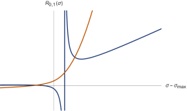
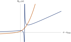
  (6)

  To understand why this condition is needed and why it is sufficient, we can limit ourselves to the pair of significative situations shown in the following plots, where the graphs of $R_0(\sigma )$ are blue curves and the graphs of $R_1(\sigma )$ are orange curves.

  

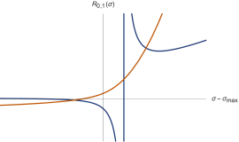
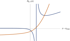
  In both cases, the blocking traction ${\sigma }_{B0}$, which corresponds the zero of $R_0$, is smaller than the blocking traction ${\sigma }_{B1}$, which is the zero of $R_1(\sigma )$. In both cases, the graphs of $R_0$ and $R_1$ have the following properties: the graph of $R_0(\sigma )$ has negative slope for and tends to $-\mathrm{\infty }$ as $\sigma$ approaches ${\sigma }_{\mathrm{asym}}$ from below; the graph of $R_1(\sigma )$ is monotone increasing and intersects the horizontal axis at ${\sigma }_{B1}>{\sigma }_{B0}$. These properties are no exception, and hold true always. A consequence of these properties is that the two graphs have a unique intersection placed on the left of the asymptote. However, while in the plot on the left-hand side, we have ${\sigma }_{\mathrm{TM}}>{\sigma }_{\max }$, in the plot on the right-hand side this is not the case. Thus, the solution on the right-hand side is not admissible. It is not difficult to realize, at this point, why the additional condition (6) is needed. This condition is simply that the orange curve stays above the blue curve at ${\sigma }_{\max }$. This condition guarantees that the two curves meet at a value of the traction smaller than ${\sigma }_{\max }$. That this condition is not only sufficient, but also necessary, follows from the fact that, in the present situation, the intersection point is on the right of ${\sigma }_{B0}$, and for $\sigma >{\sigma }_{B0}$ $R_0(\sigma )$ is decreasing while $R_1(\sigma )$ is increasing.

  The above plots are representative for . One may wonder what happens when . This is shown in the following figure.

  

  In this case, the graph of $R_0$ never crosses the horizontal axis before the asymptote. Hence the curves $R_0$ and $R_1$ intersect on the right of the asymptote. Again, all such solutions are to be discarded, since they lie to the right-hand of the vertical axis.

• The second case to be considered is . We show again two representative situations:

  

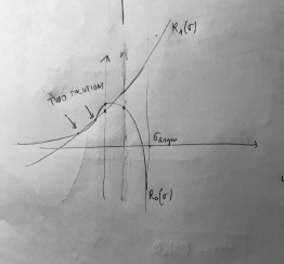
  We have exactly the same situation as before: in both cases the graphs of $R_0$ and $R_1$ meet at several points. However, the smallest intersection is, in the second case on the right of the axis ${\sigma }_{\max }$, and so treadmilling is not possible. Again, the condition is sufficient for treadmilling. However, we were not able to prove that this condition is also necessary, because we cannot assess the monotonicity of $R_0(\sigma )$ for $\sigma >{\sigma }_{B1}$. In fact, the derivative $R_0^{\prime }(\sigma )$ can be either positive or negative for $\sigma >{\sigma }_{B1}$, and hence we cannot rule out a situation like the one in the following sketch:

  

Remarks.

• The numbers $-R_0(\sigma )$ and $R_1(\sigma )$ are the growth rates at the left and right end of the bar. Their sum $R_1(\sigma )-R_0(\sigma )$ yield the total growth rate $\dot{\mathrm{\ell }}$.

• the second of (1) is obtained imposing that the traction force applied by the spring be the same as the internal stress of the bar. Its verification is one of the exercises we ask our students to do when they have two springs in serier. As one can expect, the shorter the length $\mathrm{\ell }$, the larger is the traction $\sigma$. Thus, it is not surprising that $\widehat{\mathrm{\ell }}(\sigma )$ is a monotone decreasing function. Thus, one could invert $\widehat{\mathrm{\ell }}(\sigma )$ to obtain a function $\widehat{\sigma }(\mathrm{\ell })$, to be substituted in the first of (1) to obtain a single ODE, which could be easily studied using phase-space techniques, but we prefer to proceed otherwise (see next remark ).

• the wording “blocking traction”, when referred to ${\sigma }_{B0}$ is a bit inappropriate, because the chemical potential at the clamped end is ${\mu }_0$ (an unknown). In fact, the “actual blocking traction” at the clamped end would be obtained by replacing replacing ${\mu }_1$ with ${\mu }_0$. If we did so, then the second equation of (1) would appear simpler, namely,

  $$R_0(\sigma )=-\frac{1}{B_0}\left(W^{*}(\sigma )-W^{*}({\sigma }_{B0})\right);$$

  (7)

  However, ${\sigma }_{B0}$ would depends on the unknown ${\mu }_0$. The multiplicative coefficient $\frac{{\sigma }_{\mathrm{asym}}-{\sigma }_{\max }}{{\sigma }_{\mathrm{asym}}-\sigma }$ appearing in the definition of $R_0(\sigma )$ takes care of this discrepancy. As expected, if the mobility would tend to infinity, chemical potential would be uniform, and ${\sigma }_{B0}$ would be the actual blocking traction. This is consistent with the fact that if the mobility goes to infinity, then ${\sigma }_{\max }$ tends to infinity and, as a consequence, the multiplicative coefficient $\frac{{\sigma }_{\mathrm{asym}}-{\sigma }_{\max }}{{\sigma }_{\mathrm{asym}}-\sigma }$ converges to one.

2 References

1. Rohan Abeyaratne, Eric Puntel, and Giuseppe Tomassetti. Treadmill stability of a one-dimensional actin growth model. In preparation, 2019. (note: the notation we use here differs slightly from that used in the paper).